Basics: single-structure evaluation

UPETWrapper wraps a UPET / PET-MAD checkpoint as an nvalchemi-toolkit BaseModelMixin model, so it can be driven through nvalchemi’s batched Batch data pipeline instead of ASE Atoms. This is the entry point for large-scale batched inference (see Batched evaluation) and for nvalchemi’s GPU-accelerated MD integrators (see NVT molecular dynamics).

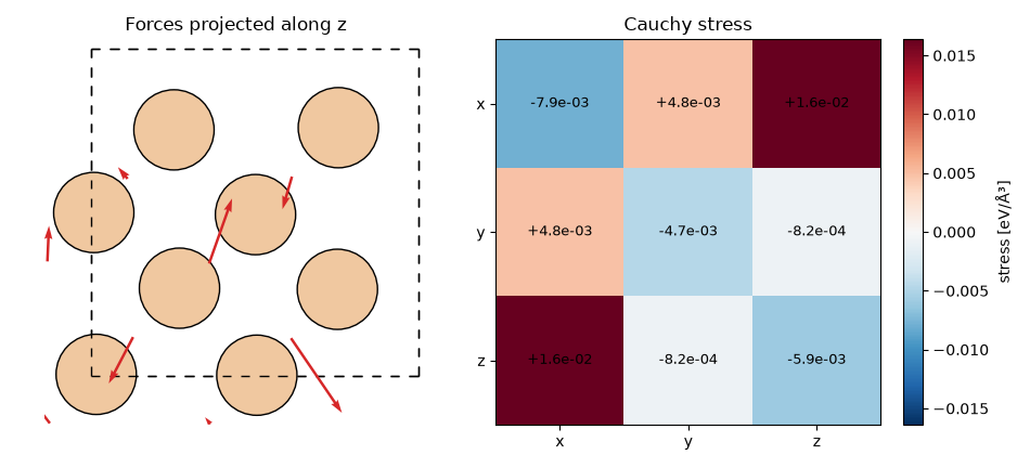
This example builds a bulk silicon cell as an ASE Atoms object, converts it to a single-graph Batch with from_atoms(), and evaluates energy, forces, and stress with UPETWrapper. Both tensorial outputs are then visualized: the forces as arrows on the projected cell, and the Cauchy stress as an annotated 3x3 map.

Note

This example requires the optional nvalchemi extra: pip install "upet[nvalchemi]".

import matplotlib.pyplot as plt
import numpy as np
import torch
from ase.build import bulk
from ase.visualize.plot import plot_atoms
from nvalchemi.data import AtomicData, Batch
from nvalchemi.neighbors import compute_neighbors

from upet.nvalchemi import UPETWrapper

Loading a checkpoint

from_checkpoint() fetches a named UPET model from HuggingFace (here the small pet-mad-xs model), or loads a local checkpoint file when checkpoint_path is given instead.

device = torch.device("cuda" if torch.cuda.is_available() else "cpu")

model = UPETWrapper.from_checkpoint(model="pet-mad-xs", version="1.6.0", device=device)

From ASE Atoms to a single-graph Batch

from_atoms() builds an AtomicData instance directly from an ASE Atoms object, carrying over positions, atomic numbers, cell and PBC. from_data_list() then promotes it to a single-graph batch.

atoms = bulk("Si", cubic=True, a=5.43, crystalstructure="diamond")

# Displace every atom slightly off its equilibrium site, so the predicted
# forces are non-zero and of comparable magnitude across the cell.
atoms.rattle(0.05, seed=0)

data = AtomicData.from_atoms(atoms, device=device)
batch = Batch.from_data_list([data], device=device)

Neighbor list and evaluation

compute_neighbors() is the one-shot convenience function for populating a batch’s neighbor list outside a dynamics loop; model.model_config.neighbor_config already encodes the cutoff and list format the model expects.

compute_neighbors(batch, config=model.model_config.neighbor_config)

outputs = model(batch)

print(f"Energy : {outputs['energy'].item():+.4f} eV")
print(f"Forces :\n{outputs['forces'].detach().cpu().numpy()}")
print(f"Stress :\n{outputs['stress'].squeeze(0).detach().cpu().numpy()}")

Energy : -46.8500 eV
Forces :
[[-0.6098818   0.79013574 -0.30601698]
 [-0.55659235 -1.0620064   0.96056247]
 [ 0.03621662  0.81610477 -0.3269433 ]
 [-0.22019836  0.2661117  -1.3370566 ]
 [-0.12413108  0.15760766 -0.23730144]
 [ 1.1662254  -1.7095635  -0.4695834 ]
 [ 0.5255206   1.4886923   1.489167  ]
 [-0.2171591  -0.74708265  0.22717234]]
Stress :
[[-0.00786457  0.00477575  0.0163688 ]
 [ 0.00477575 -0.00465882 -0.0008237 ]
 [ 0.0163688  -0.0008237  -0.00593601]]

Visualizing the forces and the stress tensor

AtomicData.from_atoms keeps the atom ordering of the Atoms object, so the force rows line up with atoms and can be drawn straight onto a projection of the cell. The left panel looks down the z axis and overlays the in-plane force components as arrows; the right panel shows the full Cauchy stress tensor, whose off-diagonal (shear) components are non-zero because the rattle breaks the cubic symmetry of the ideal diamond cell.

positions = atoms.get_positions()
forces = outputs["forces"].detach().cpu().numpy()
stress = outputs["stress"].squeeze(0).detach().cpu().numpy()

# Scale the arrows so the largest one spans ~1.5 Å on the plot, whatever
# the force magnitudes happen to be.
arrow_scale = np.linalg.norm(forces[:, :2], axis=1).max() / 1.5

fig, (ax_forces, ax_stress) = plt.subplots(1, 2, figsize=(9.5, 4.2))

plot_atoms(atoms, ax_forces, radii=0.6, show_unit_cell=2)
ax_forces.quiver(
    positions[:, 0],
    positions[:, 1],
    forces[:, 0],
    forces[:, 1],
    color="tab:red",
    angles="xy",
    scale_units="xy",
    scale=arrow_scale,
    width=0.007,
)
ax_forces.set_title("Forces projected along z")
ax_forces.set_xlabel("x [Å]")
ax_forces.set_ylabel("y [Å]")

limit = np.abs(stress).max()
image = ax_stress.imshow(stress, cmap="RdBu_r", vmin=-limit, vmax=limit)
for i in range(3):
    for j in range(3):
        ax_stress.text(
            j, i, f"{stress[i, j]:+.1e}", ha="center", va="center", fontsize=9
        )
labels = ["x", "y", "z"]
ax_stress.set_xticks(range(3), labels)
ax_stress.set_yticks(range(3), labels)
ax_stress.set_title("Cauchy stress")
fig.colorbar(image, ax=ax_stress, label="stress [eV/ų]", fraction=0.046)

fig.tight_layout()
plt.show()