NPT molecular dynamics

NPT samples the isothermal-isobaric ensemble via a Martyna-Tobias-Klein barostat coupled to a Nosé-Hoover thermostat, so both the atomic positions and the simulation cell evolve. This example runs it on a silicon supercell at 300 K and 1 bar, with UPETWrapper supplying forces and stress. The three quantities the two barostats and the thermostat control – temperature, cell volume, and instantaneous pressure – are recorded at every step and plotted together.

Note

This example requires the optional nvalchemi extra: pip install "upet[nvalchemi]".

from collections import defaultdict

import matplotlib.pyplot as plt
import numpy as np
import torch
from ase import units
from ase.build import bulk
from nvalchemi.data import AtomicData, Batch
from nvalchemi.dynamics import NPT, DynamicsStage, initialize_velocities
from nvalchemi.hooks import NeighborListHook, extract_dynamics_scalars
from nvalchemi.neighbors import compute_neighbors

from upet.nvalchemi import UPETWrapper


device = torch.device("cuda" if torch.cuda.is_available() else "cpu")
model = UPETWrapper.from_checkpoint(model="pet-mad-xs", version="1.6.0", device=device)

atoms = bulk("Si", cubic=True, a=5.43, crystalstructure="diamond").repeat((2, 2, 2))
data = AtomicData.from_atoms(atoms, device=device)

# The integrators write model outputs back into the batch fields that already
# exist and silently skip the ones that don't, while `AtomicData.from_atoms`
# only fills the fields the `Atoms` object itself carries -- so the output
# buffers have to be allocated up front.
data.energy = torch.zeros(1, 1, device=device)
data.forces = torch.zeros_like(data.positions)
data.stress = torch.zeros(1, 3, 3, device=device)

batch = Batch.from_data_list([data], device=device)
compute_neighbors(batch, config=model.model_config.neighbor_config)

# nvalchemi's pressure follows the same eV/ų convention as its Cauchy
# stress output, matching ASE's internal unit system for stress.
bar = 1e-4 * units.GPa

Recording the trajectory

nvalchemi runs the whole loop inside run(), so anything to be plotted afterwards has to be collected while the loop is running. A hook registered at AFTER_STEP is the nvalchemi counterpart of ASE’s dyn.attach(logger, interval=1). extract_dynamics_scalars() supplies the standard observables (potential energy, max force norm, temperature); under NPT the cell moves too, so this recorder also derives the volume from batch.cell and the hydrostatic pressure from the trace of the Cauchy stress.

class TrajectoryRecorder:
    """Append the per-step scalar observables to a history dict."""

    def __init__(self):
        self.frequency = 1  # fire on every step
        self.stage = DynamicsStage.AFTER_STEP
        self.history: dict[str, list[float]] = defaultdict(list)

    def __call__(self, ctx, stage):
        self.history["step"].append(ctx.step_count)
        for key, value in extract_dynamics_scalars(ctx).items():
            self.history[key].append(value)

        cell = ctx.batch.cell
        self.history["volume"].append(torch.linalg.det(cell).abs().item())

        # p = -tr(sigma) / 3, converted from eV/ų to bar
        stress = ctx.batch.stress.squeeze(0)
        pressure = -torch.diagonal(stress).sum() / 3.0
        self.history["pressure"].append(pressure.item() / bar)


T_TARGET = 300.0  # K

temperature = torch.full((batch.num_graphs,), T_TARGET, device=device)
initialize_velocities(
    batch.velocities, batch.atomic_masses, temperature, batch.batch_idx.int()
)

TIMESTEP = 1.0  # fs
P_TARGET_BAR = 1.0

recorder = TrajectoryRecorder()
npt = NPT(
    model=model,
    dt=TIMESTEP,
    temperature=T_TARGET,
    pressure=P_TARGET_BAR * bar,
    barostat_time=100.0,
    thermostat_time=25.0,
    n_steps=200,
    hooks=[
        NeighborListHook(
            model.model_config.neighbor_config,
            skin=0.5,
            stage=DynamicsStage.BEFORE_COMPUTE,
        ),
        recorder,
    ],
)

# The first integrator step already reads the forces, so the batch needs one
# model evaluation before the loop starts.
npt.compute(batch)
batch = npt.run(batch)

print(f"Ran {npt.step_count} NPT steps")
print(f"Energy : {batch.energy.item():+.4f} eV")
print(f"Volume : {torch.linalg.det(batch.cell).abs().item():.2f} ų")

Ran 200 NPT steps
Energy : -375.3653 eV
Volume : 1289.07 ų

Thermostat and barostat behaviour

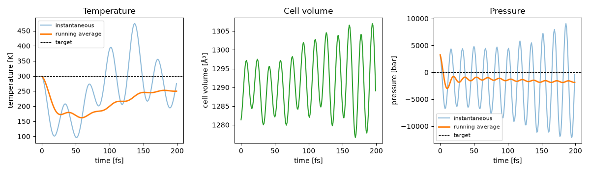
This is a 200 fs run against a 25 fs thermostat time and a 100 fs barostat time, so what the plots show is the start of the coupling transient, not converged NPT sampling. Read it that way:

• The temperature swings between roughly 100 K and 500 K. The initial velocities are drawn at 300 K on the ideal lattice, so the crystal starts with no potential energy of its own and rings coherently as energy sloshes between the kinetic and potential reservoirs; a few thermostat times are needed before that ringing is damped out.

• The cell volume drifts upward and oscillates with the same period – the barostat is still responding to the initial pressure imbalance.

• The instantaneous pressure of a 64-atom cell covers thousands of bar. Pressure in a small system is dominated by fluctuations, so only the running average can be compared against the 1 bar setpoint, and after two barostat times it has not reached it yet.

Equilibrating this system properly means running for tens of picoseconds and discarding the transient before averaging; 200 steps is chosen here to keep the example fast.

times = np.asarray(recorder.history["step"]) * TIMESTEP
temperatures = np.asarray(recorder.history["temperature"])
pressures = np.asarray(recorder.history["pressure"])


def running_average(values):
    return np.cumsum(values) / np.arange(1, len(values) + 1)


fig, (ax_temperature, ax_volume, ax_pressure) = plt.subplots(1, 3, figsize=(12, 3.5))

ax_temperature.plot(times, temperatures, alpha=0.5, label="instantaneous")
ax_temperature.plot(times, running_average(temperatures), lw=2, label="running average")
ax_temperature.axhline(T_TARGET, color="k", ls="--", lw=0.8, label="target")
ax_temperature.set_xlabel("time [fs]")
ax_temperature.set_ylabel("temperature [K]")
ax_temperature.set_title("Temperature")
ax_temperature.legend(fontsize=8)

ax_volume.plot(times, recorder.history["volume"], color="tab:green")
ax_volume.set_xlabel("time [fs]")
ax_volume.set_ylabel("cell volume [ų]")
ax_volume.set_title("Cell volume")

ax_pressure.plot(times, pressures, alpha=0.5, label="instantaneous")
ax_pressure.plot(times, running_average(pressures), lw=2, label="running average")
ax_pressure.axhline(P_TARGET_BAR, color="k", ls="--", lw=0.8, label="target")
ax_pressure.set_xlabel("time [fs]")
ax_pressure.set_ylabel("pressure [bar]")
ax_pressure.set_title("Pressure")
ax_pressure.legend(fontsize=8)

fig.tight_layout()
plt.show()