NVE molecular dynamics

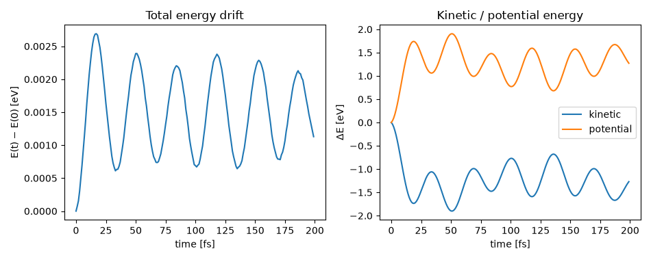
NVE integrates Newton’s equations of motion with the velocity Verlet algorithm, conserving the total energy. This example runs it on a silicon supercell with UPETWrapper supplying conservative forces. Kinetic and potential energy are recorded at every step: they exchange back and forth as the crystal equilibrates, while their sum stays flat up to integration error.

Note

This example requires the optional nvalchemi extra: pip install "upet[nvalchemi]".

from collections import defaultdict

import matplotlib.pyplot as plt
import numpy as np
import torch
from ase import units
from ase.build import bulk
from nvalchemi.data import AtomicData, Batch
from nvalchemi.dynamics import NVE, DynamicsStage, initialize_velocities
from nvalchemi.hooks import NeighborListHook, extract_dynamics_scalars
from nvalchemi.neighbors import compute_neighbors

from upet.nvalchemi import UPETWrapper


device = torch.device("cuda" if torch.cuda.is_available() else "cpu")
model = UPETWrapper.from_checkpoint(model="pet-mad-xs", version="1.6.0", device=device)

atoms = bulk("Si", cubic=True, a=5.43, crystalstructure="diamond").repeat((2, 2, 2))
data = AtomicData.from_atoms(atoms, device=device)

# The integrators write model outputs back into the batch fields that already
# exist and silently skip the ones that don't, while `AtomicData.from_atoms`
# only fills the fields the `Atoms` object itself carries -- so the output
# buffers have to be allocated up front.
data.energy = torch.zeros(1, 1, device=device)
data.forces = torch.zeros_like(data.positions)

batch = Batch.from_data_list([data], device=device)
compute_neighbors(batch, config=model.model_config.neighbor_config)

Recording the trajectory

nvalchemi runs the whole loop inside run(), so anything to be plotted afterwards has to be collected while the loop is running. A hook registered at AFTER_STEP is the nvalchemi counterpart of ASE’s dyn.attach(logger, interval=1). extract_dynamics_scalars() pulls the standard observables (potential energy, max force norm, temperature) off the batch, so the hook itself only has to accumulate them.

class TrajectoryRecorder:
    """Append the per-step scalar observables to a history dict."""

    def __init__(self):
        self.frequency = 1  # fire on every step
        self.stage = DynamicsStage.AFTER_STEP
        self.history: dict[str, list[float]] = defaultdict(list)

    def __call__(self, ctx, stage):
        self.history["step"].append(ctx.step_count)
        for key, value in extract_dynamics_scalars(ctx).items():
            self.history[key].append(value)


temperature = torch.full((batch.num_graphs,), 300.0, device=device)
initialize_velocities(
    batch.velocities, batch.atomic_masses, temperature, batch.batch_idx.int()
)

# `NeighborListHook` rebuilds the neighbor list during the run, once an atom
# has moved further than the `skin` buffer.
TIMESTEP = 1.0  # fs

recorder = TrajectoryRecorder()
nve = NVE(
    model=model,
    dt=TIMESTEP,
    n_steps=200,
    hooks=[
        NeighborListHook(
            model.model_config.neighbor_config,
            skin=0.5,
            stage=DynamicsStage.BEFORE_COMPUTE,
        ),
        recorder,
    ],
)

# The first integrator step already reads the forces, so the batch needs one
# model evaluation before the loop starts.
nve.compute(batch)
batch = nve.run(batch)

print(f"Ran {nve.step_count} NVE steps")
print(f"Energy : {batch.energy.item():+.4f} eV")

Ran 200 NVE steps
Energy : -376.6247 eV

Energy conservation

extract_dynamics_scalars reports the temperature rather than the kinetic energy, but the two are related by equipartition over the 3N degrees of freedom, KE = (3/2) N k_B T, which is exactly the definition nvalchemi uses – so the kinetic energy can be recovered without touching the velocities.

The starting configuration is the ideal diamond lattice with velocities drawn at 300 K, so all of the energy is initially kinetic. Half of it converts to potential energy within the first few tens of femtoseconds – the usual equipartition transient – after which the two oscillate about their equilibrium partition. The total energy is the quantity to watch: it stays flat, which is what makes the forces usable for microcanonical sampling.

times = np.asarray(recorder.history["step"]) * TIMESTEP
e_pot = np.asarray(recorder.history["energy"])
temperatures = np.asarray(recorder.history["temperature"])
e_kin = 1.5 * len(atoms) * units.kB * temperatures
e_tot = e_pot + e_kin

fig, (ax_total, ax_split) = plt.subplots(1, 2, figsize=(9.5, 3.8))

ax_total.plot(times, e_tot - e_tot[0])
ax_total.set_xlabel("time [fs]")
ax_total.set_ylabel("E(t) − E(0) [eV]")
ax_total.set_title("Total energy drift")

ax_split.plot(times, e_kin - e_kin[0], label="kinetic")
ax_split.plot(times, e_pot - e_pot[0], label="potential")
ax_split.set_xlabel("time [fs]")
ax_split.set_ylabel("ΔE [eV]")
ax_split.set_title("Kinetic / potential energy")
ax_split.legend()

fig.tight_layout()
plt.show()