Advanced neighbor list usage

Accurately calculating forces as derivatives from energy is crucial for predicting system dynamics as well as in training machine learning models. In systems where forces are derived from the gradients of the potential energy, it is essential that the distance calculations between particles are included in the computational graph. This ensures that the force computations respect the dependencies between particle positions and distances, allowing for accurate gradients during backpropagation.

Visualization of the data flow to compute the energy from the cell, positions and charges through a neighborlist calculator and the potential calculator. All operations on the red line have to be tracked to obtain the correct computation of derivatives on the positions.

In this tutorial, we demonstrate two methods for maintaining differentiability when computing distances between particles. The first method manually recomputes distances within the computational graph using positions, cell information, and neighbor shifts, making it suitable for any neighbor list code.

The second method uses a backpropagable neighbor list from the vesin-torch library, which automatically ensures that the distance calculations remain differentiable.

Note

While both approaches yield the same result, a backpropagable neighbor list is generally preferred because it eliminates the need to manually recompute distances. This not only simplifies your code but also improves performance.

from typing import Optional

import ase
import chemiscope
import matplotlib.pyplot as plt
import numpy as np
import torch
import vesin
import vesin.torch

import torchpme
from torchpme.tuning import tune_pme

The test system

As a test system, we use a 2x2x2 supercell of an CsCl crystal in a cubic cell.

dtype = torch.float64
atoms_unitcell = ase.Atoms(
    symbols=["Cs", "Cl"],
    positions=np.array([(0, 0, 0), (0.5, 0.5, 0.5)]),
    cell=np.eye(3),
    pbc=torch.tensor([True, True, True]),
)
charges_unitcell = np.array([1.0, -1.0])

atoms = atoms_unitcell.repeat([2, 2, 2])
charges = np.tile(charges_unitcell, 2 * 2 * 2)

We now slightly displace the atoms from their initial positions randomly based on a Gaussian distribution with a width of 0.1 Å to create non-zero forces.

atoms.rattle(stdev=0.1)

chemiscope.show(
    frames=[atoms],
    mode="structure",
    settings=chemiscope.quick_settings(structure_settings={"unitCell": True}),
)

×

Tune paramaters

Based on our system we will first tune the PME parameters for an accurate computation. We first convert the positions, charges and the cell from NumPy arrays into torch tensors and compute the summed squared charges.

positions = torch.from_numpy(atoms.positions)
charges = torch.from_numpy(charges).unsqueeze(1)
cell = torch.from_numpy(atoms.cell.array)

sum_squared_charges = float(torch.sum(charges**2))
cutoff = 4.4
nl = vesin.torch.NeighborList(cutoff=cutoff, full_list=False)
neighbor_indices, neighbor_distances = nl.compute(
    points=positions.to(dtype=torch.float64, device="cpu"),
    box=cell.to(dtype=dtype, device="cpu"),
    periodic=True,
    quantities="Pd",
)

smearing, pme_params, _ = tune_pme(
    charges=charges,
    cell=cell,
    positions=positions,
    cutoff=cutoff,
    neighbor_indices=neighbor_indices,
    neighbor_distances=neighbor_distances,
)

The tuning found the following best values for our system.

print("smearing:", smearing)
print("PME parameters:", pme_params)
print("cutoff:", cutoff)

smearing: 1.1069526756106463
PME parameters: {'interpolation_nodes': 4, 'mesh_spacing': 0.5714285714285714}
cutoff: 4.4

Generic Neighborlist

One usual workflow is to compute the distance vectors using default tools like the the default (NumPy) version of the vesin neighbor list.

nl = vesin.NeighborList(cutoff=cutoff, full_list=False)
neighbor_indices, S = nl.compute(
    points=atoms.positions, box=atoms.cell.array, periodic=True, quantities="PS"
)

We now define a function that (re-)computes the distances in a way that torch can track these operations.

def distances(
    positions: torch.Tensor,
    neighbor_indices: torch.Tensor,
    cell: Optional[torch.Tensor] = None,
    neighbor_shifts: Optional[torch.Tensor] = None,
) -> torch.Tensor:
    """Compute pairwise distances."""
    atom_is = neighbor_indices[:, 0]
    atom_js = neighbor_indices[:, 1]

    pos_is = positions[atom_is]
    pos_js = positions[atom_js]

    distance_vectors = pos_js - pos_is

    if cell is not None and neighbor_shifts is not None:
        shifts = neighbor_shifts.type(cell.dtype)
        distance_vectors += shifts @ cell
    elif cell is not None and neighbor_shifts is None:
        raise ValueError("Provided `cell` but no `neighbor_shifts`.")
    elif cell is None and neighbor_shifts is not None:
        raise ValueError("Provided `neighbor_shifts` but no `cell`.")

    return torch.linalg.norm(distance_vectors, dim=1)

To use this function we now the tracking of operations by setting the requires_grad property to True.

positions.requires_grad = True

neighbor_indices = torch.from_numpy(neighbor_indices.astype(int))
neighbor_shifts = torch.from_numpy(S)

Now, we start to re-compute the distances

neighbor_distances = distances(
    positions=positions,
    neighbor_indices=neighbor_indices,
    cell=cell,
    neighbor_shifts=neighbor_shifts,
)

and initialize a PMECalculator instance using a CoulombPotential to compute the potential.

pme = torchpme.PMECalculator(
    potential=torchpme.CoulombPotential(smearing=smearing),
    **pme_params,
)
potential = pme(
    charges=charges,
    cell=cell,
    positions=positions,
    neighbor_indices=neighbor_indices,
    neighbor_distances=neighbor_distances,
)

print(potential)

tensor([[-0.8874],
        [ 1.2554],
        [-0.9274],
        [ 1.4907],
        [-0.7261],
        [ 0.7836],
        [-0.8839],
        [ 0.8997],
        [-0.9603],
        [ 1.0151],
        [-1.0800],
        [ 1.3655],
        [-1.0228],
        [ 0.6690],
        [-1.1581],
        [ 0.8331]], dtype=torch.float64, grad_fn=<MulBackward0>)

The energy is given by the scalar product of the potential with the charges.

energy = charges.T @ potential

Finally, we can compute and print the forces in CGS units as erg/Å.

forces = torch.autograd.grad(-1.0 * energy, positions)[0]

print(forces)

tensor([[-0.9484, -1.4864,  0.9129],
        [ 0.1350, -0.6500,  0.4235],
        [-0.0230, -1.4964, -0.1962],
        [-0.3949, -0.3494,  0.1579],
        [-0.0038,  0.9212,  1.0006],
        [ 0.2718,  0.2613, -0.4679],
        [-1.2057,  0.9323, -1.0406],
        [-0.3698,  0.5807,  0.5612],
        [ 0.5696, -1.1072,  0.0541],
        [ 0.6476,  0.4007, -0.4058],
        [ 0.5322,  0.1812, -0.3541],
        [ 0.5632,  0.4293,  0.3243],
        [ 0.4923,  0.5976, -0.6239],
        [ 0.0734,  0.1513,  0.0368],
        [-0.3666,  0.8548, -0.5614],
        [ 0.0273, -0.2203,  0.1787]], dtype=torch.float64)

Backpropagable Neighborlist

We now repeat the computation of the forces, but instead of using a generic neighbor list and our custom distances function, we directly use a neighbor list function that tracks the operations, as implemented by the vesin-torch library.

We first detach and clone the position tensor to create a new computational graph

positions_new = positions.detach().clone()
positions_new.requires_grad = True

and create new distances in a similar manner as above.

nl = vesin.torch.NeighborList(cutoff=cutoff, full_list=False)
neighbor_indices_new, d = nl.compute(
    points=positions_new, box=cell, periodic=True, quantities="Pd"
)

Following the same steps as above, we compute the forces.

potential_new = pme(
    charges=charges,
    cell=cell,
    positions=positions_new,
    neighbor_indices=neighbor_indices_new,
    neighbor_distances=d,
)

energy_new = charges.T @ potential_new

forces_new = torch.autograd.grad(-1.0 * energy_new, positions_new)[0]

print(forces_new)

tensor([[-0.9484, -1.4864,  0.9129],
        [ 0.1350, -0.6500,  0.4235],
        [-0.0230, -1.4964, -0.1962],
        [-0.3949, -0.3494,  0.1579],
        [-0.0038,  0.9212,  1.0006],
        [ 0.2718,  0.2613, -0.4679],
        [-1.2057,  0.9323, -1.0406],
        [-0.3698,  0.5807,  0.5612],
        [ 0.5696, -1.1072,  0.0541],
        [ 0.6476,  0.4007, -0.4058],
        [ 0.5322,  0.1812, -0.3541],
        [ 0.5632,  0.4293,  0.3243],
        [ 0.4923,  0.5976, -0.6239],
        [ 0.0734,  0.1513,  0.0368],
        [-0.3666,  0.8548, -0.5614],
        [ 0.0273, -0.2203,  0.1787]], dtype=torch.float64)

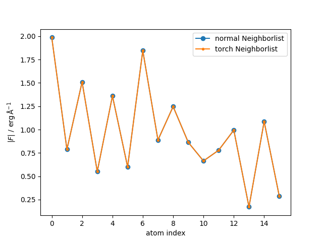
The forces are the same as those we printed above. For better comparison, we can also plot the scalar force for each method.

plt.plot(torch.linalg.norm(forces, dim=1), "o-", label="normal Neighborlist")
plt.plot(torch.linalg.norm(forces_new, dim=1), ".-", label="torch Neighborlist")
plt.legend()

plt.xlabel("atom index")
plt.ylabel(r"$|F|~/~\mathrm{erg\,Å^{-1}}$")

plt.show()