Parameter tuning for range-separated models

Authors:

Michele Ceriotti @ceriottm

Metods to compute efficiently a long-range potential \(v(r)\) usually rely on partitioning it into a short-range part, evaluated as a sum over neighbor pairs, and a long-range part evaluated in reciprocal space

\[v(r)= v_{\mathrm{SR}}(r) + v_{\mathrm{LR}}(r)\]

The overall cost depend on the balance of multiple factors, that we summarize here briefly to explain how the cost of evaluating \(v(r)\) can be minimized, either manually or automatically.

Import modules

import ase
import matplotlib as mpl
import matplotlib.pyplot as plt
import numpy as np
import torch
import vesin.torch as vesin

import torchpme
from torchpme.tuning.pme import PMEErrorBounds, tune_pme
from torchpme.tuning.tuner import TuningTimings

device = "cpu"
dtype = torch.float64
rng = torch.Generator()
rng.manual_seed(42)

# get_ipython().run_line_magic("matplotlib", "inline")  # type: ignore # noqa

<torch._C.Generator object at 0x7f8fb1d9e4b0>

Set up a test system, a supercell containing atoms with a NaCl structure

madelung_ref = 1.7475645946
structure = ase.Atoms(
    positions=[
        [0, 0, 0],
        [1, 0, 0],
        [0, 1, 0],
        [1, 1, 0],
        [0, 0, 1],
        [1, 0, 1],
        [0, 1, 1],
        [1, 1, 1],
    ],
    cell=[2, 2, 2],
    symbols="NaClClNaClNaNaCl",
)
structure = structure.repeat([2, 2, 2])
num_formula_units = len(structure) // 2

# Uncomment these to add a displacement (energy won't match the Madelung constant)
# displacement = torch.normal(
#    mean=0.0, std=2.5e-1, size=(len(structure), 3), generator=rng
# )
# structure.positions += displacement.numpy()

positions = torch.from_numpy(structure.positions).to(device=device, dtype=dtype)
cell = torch.from_numpy(structure.cell.array).to(device=device, dtype=dtype)

charges = torch.tensor(
    [[1.0], [-1.0], [-1.0], [1.0], [-1.0], [1.0], [1.0], [-1.0]]
    * (len(structure) // 8),
    dtype=dtype,
    device=device,
).reshape(-1, 1)

# Uncomment these to randomize charges (energy won't match the Madelung constant)
# charges += torch.normal(mean=0.0, std=1e-1, size=(len(charges), 1), generator=rng)

We also need to evaluate the neighbor list; this is usually pre-computed by the code that calls torch-pme, and entails the first key parameter: the cutoff used to compute the real-space potential \(v_\mathrm{SR}(r)\)

max_cutoff = 16.0

# use `vesin`
nl = vesin.NeighborList(cutoff=max_cutoff, full_list=False)
i, j, S, d = nl.compute(points=positions, box=cell, periodic=True, quantities="ijSd")
neighbor_indices = torch.stack([i, j], dim=1)
neighbor_shifts = S
neighbor_distances = d

Demonstrate errors and timings for PME

To set up a PME calculation, we need to define its basic parameters and setup a few preliminary quantities.

The PME calculator has a few further parameters: smearing, that determines aggressive is the smoothing of the point charges. This makes the reciprocal-space part easier to compute, but makes \(v_\mathrm{SR}(r)\) decay more slowly, and error that we shall investigate further later on. The mesh parameters involve both the spacing and the order of the interpolation used. Note that here we use CoulombPotential, that computes a simple \(1/r\) electrostatic interaction.

smearing = 1.0
pme_params = {"mesh_spacing": 1.0, "interpolation_nodes": 4}

pme = torchpme.PMECalculator(
    potential=torchpme.CoulombPotential(smearing=smearing),
    **pme_params,  # type: ignore[arg-type]
)
pme.to(device=device, dtype=dtype)

PMECalculator(
  (potential): CoulombPotential()
  (kspace_filter): KSpaceFilter(
    (kernel): CoulombPotential()
  )
  (mesh_interpolator): MeshInterpolator()
)

Run the calculator

We combine the structure data and the neighbor list information to compute the potential at the particle positions, and then the energy

potential = pme(
    charges=charges,
    cell=cell,
    positions=positions,
    neighbor_indices=neighbor_indices,
    neighbor_distances=neighbor_distances,
)

energy = charges.T @ potential
madelung = (-energy / num_formula_units).flatten().item()

Compute error bounds (and timings)

Here we calculate the potential energy of the system, and compare it with the madelung constant to calculate the error. This is the actual error. Then we use the torchpme.tuning.pme.PMEErrorBounds to calculate the error bound for PME. Error bounds are computed explicitly for a target structure

error_bounds = PMEErrorBounds(charges, cell, positions)

estimated_error = error_bounds(
    cutoff=max_cutoff, smearing=smearing, **pme_params
).item()

… and a similar class can be used to estimate the timings, that are assessed based on a calculator (that should be initialized with the same parameters)

timings = TuningTimings(
    charges,
    cell,
    positions,
    neighbor_indices=neighbor_indices,
    neighbor_distances=neighbor_distances,
    run_backward=True,
)
estimated_timing = timings(pme)

The error bound is estimated for the force acting on atoms, and is expressed in force units - hence, the comparison with the Madelung constant error can only be qualitative.

print(
    f"""
Computed madelung constant: {madelung}
Actual error: {madelung - madelung_ref}
Estimated error: {estimated_error}
Timing: {estimated_timing} seconds
"""
)

Computed madelung constant: 1.7475645946331768
Actual error: 3.317679464487355e-11
Estimated error: 0.0013000359004761823
Timing: 0.059277408999989234 seconds

Optimizing the parameters of PME

There are many parameters that enter the implementation of a range-separated calculator like PME, and it is necessary to optimize them to obtain the best possible accuracy/cost tradeoff. In most practical use cases, the cutoff is dictated by the external calculator and is treated as a fixed parameter. In cases where performance is critical, one may want to optimize this separately, which can be achieved easily with a grid or binary search.

We can set up easily a brute-force evaluation of the error as a function of these parameters, and use it to guide the design of a more sophisticated optimization protocol.

def filter_neighbors(cutoff, neighbor_indices, neighbor_distances):
    assert cutoff <= max_cutoff

    filter_idx = torch.where(neighbor_distances <= cutoff)

    return neighbor_indices[filter_idx], neighbor_distances[filter_idx]


def timed_madelung(cutoff, smearing, mesh_spacing, interpolation_nodes, device, dtype):
    filter_indices, filter_distances = filter_neighbors(
        cutoff, neighbor_indices, neighbor_distances
    )

    pme = torchpme.PMECalculator(
        potential=torchpme.CoulombPotential(smearing=smearing),
        mesh_spacing=mesh_spacing,
        interpolation_nodes=interpolation_nodes,
    )
    pme.to(device=device, dtype=dtype)
    potential = pme(
        charges=charges,
        cell=cell,
        positions=positions,
        neighbor_indices=filter_indices,
        neighbor_distances=filter_distances,
    )
    energy = charges.T @ potential
    madelung = (-energy / num_formula_units).flatten().item()

    timings = TuningTimings(
        charges,
        cell,
        positions,
        neighbor_indices=filter_indices,
        neighbor_distances=filter_distances,
        run_backward=True,
        n_warmup=1,
        n_repeat=4,
    )
    estimated_timing = timings(pme)
    return madelung, estimated_timing


smearing_grid = torch.logspace(-1, 0.5, 8)
spacing_grid = torch.logspace(-1, 0.5, 9)
results = np.zeros((len(smearing_grid), len(spacing_grid)))
timings = np.zeros((len(smearing_grid), len(spacing_grid)))
bounds = np.zeros((len(smearing_grid), len(spacing_grid)))
for ism, smearing in enumerate(smearing_grid):
    for isp, spacing in enumerate(spacing_grid):
        results[ism, isp], timings[ism, isp] = timed_madelung(
            8.0, smearing, spacing, 4, device, dtype
        )
        bounds[ism, isp] = error_bounds(8.0, smearing, spacing, 4)

/home/runner/work/torch-pme/torch-pme/src/torchpme/potentials/potential.py:44: UserWarning: To copy construct from a tensor, it is recommended to use sourceTensor.clone().detach() or sourceTensor.clone().detach().requires_grad_(True), rather than torch.tensor(sourceTensor).
  "smearing", torch.tensor(smearing, dtype=torch.float64)
/home/runner/work/torch-pme/torch-pme/src/torchpme/tuning/pme.py:263: UserWarning: To copy construct from a tensor, it is recommended to use sourceTensor.clone().detach() or sourceTensor.clone().detach().requires_grad_(True), rather than torch.tensor(sourceTensor).
  smearing = torch.tensor(smearing)
/home/runner/work/torch-pme/torch-pme/src/torchpme/tuning/pme.py:264: UserWarning: To copy construct from a tensor, it is recommended to use sourceTensor.clone().detach() or sourceTensor.clone().detach().requires_grad_(True), rather than torch.tensor(sourceTensor).
  mesh_spacing = torch.tensor(mesh_spacing)

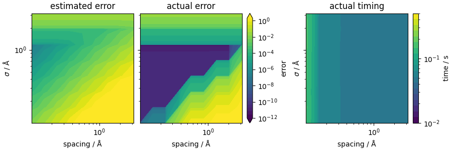
We now plot the error landscape. The estimated error can be seen as a upper bound of the actual error. Though the magnitude of the estimated error is higher than the actual error, the trend is the same. Also, from the timing results, we can see that the timing increases as the spacing decreases, while the smearing does not affect the timing, because the interactions are computed up to the fixed cutoff regardless of whether \(v_\mathrm{sr}(r)\) is negligible or large.

vmin = 1e-12
vmax = 2
levels = np.geomspace(vmin, vmax, 30)

fig, ax = plt.subplots(1, 3, figsize=(9, 3), sharey=True, constrained_layout=True)
contour = ax[0].contourf(
    spacing_grid,
    smearing_grid,
    bounds,
    vmin=vmin,
    vmax=vmax,
    levels=levels,
    norm=mpl.colors.LogNorm(),
    extend="both",
)
ax[0].set_xscale("log")
ax[0].set_yscale("log")
ax[0].set_ylabel(r"$\sigma$ / Å")
ax[0].set_xlabel(r"spacing / Å")
ax[0].set_title("estimated error")
cbar = fig.colorbar(contour, ax=ax[1], label="error")
cbar.ax.set_yscale("log")

contour = ax[1].contourf(
    spacing_grid,
    smearing_grid,
    np.abs(results - madelung_ref),
    vmin=vmin,
    vmax=vmax,
    levels=levels,
    norm=mpl.colors.LogNorm(),
    extend="both",
)
ax[1].set_xscale("log")
ax[1].set_yscale("log")
ax[1].set_xlabel(r"spacing / Å")
ax[1].set_title("actual error")

contour = ax[2].contourf(
    spacing_grid,
    smearing_grid,
    timings,
    levels=np.geomspace(1e-2, 5e-1, 20),
    norm=mpl.colors.LogNorm(),
)
ax[2].set_xscale("log")
ax[2].set_yscale("log")
ax[2].set_ylabel(r"$\sigma$ / Å")
ax[2].set_xlabel(r"spacing / Å")
ax[2].set_title("actual timing")
cbar = fig.colorbar(contour, ax=ax[2], label="time / s")
cbar.ax.set_yscale("log")

Optimizing the smearing

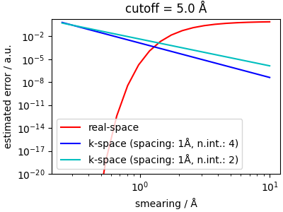
The error is a sum of an error on the real-space evaluation of the short-range potential, and of a long-range error. Considering the cutoff as given, the short-range error is determined easily by how quickly \(v_\mathrm{sr}(r)\) decays to zero, which depends on the Gaussian smearing.

smearing_grid = torch.logspace(-0.6, 1, 20)
err_vsr_grid = error_bounds.err_rspace(smearing_grid, torch.tensor([5.0]))
err_vlr_grid_4 = [
    error_bounds.err_kspace(
        torch.tensor([s]), torch.tensor([1.0]), torch.tensor([4], dtype=int)
    )
    for s in smearing_grid
]
err_vlr_grid_2 = [
    error_bounds.err_kspace(
        torch.tensor([s]), torch.tensor([1.0]), torch.tensor([3], dtype=int)
    )
    for s in smearing_grid
]

fig, ax = plt.subplots(1, 1, figsize=(4, 3), constrained_layout=True)
ax.loglog(smearing_grid, err_vsr_grid, "r-", label="real-space")
ax.loglog(smearing_grid, err_vlr_grid_4, "b-", label="k-space (spacing: 1Å, n.int.: 4)")
ax.loglog(smearing_grid, err_vlr_grid_2, "c-", label="k-space (spacing: 1Å, n.int.: 2)")
ax.set_ylabel(r"estimated error / a.u.")
ax.set_xlabel(r"smearing / Å")
ax.set_title("cutoff = 5.0 Å")
ax.set_ylim(1e-20, 2)
ax.legend()

<matplotlib.legend.Legend object at 0x7f8ed09e8a50>

Given the simple, monotonic and fast-varying trend for the real-space error, it is easy to pick the optimal smearing as the value corresponding to roughly half of the target error -e.g. for a target accuracy of \(1e^{-5}\), one would pick a smearing of about 1Å. Given that usually there is a cost/accuracy tradeoff, and smaller smearings make the reciprocal-space evaluation more costly, the largest smearing is the best choice here.

Optimizing mesh and interpolation order

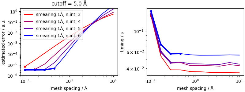
Once the smearing value that gives an acceptable accuracy for the real-space component has been determined, there may be other parameters that need to be optimized. One way to do this is to perform a grid search, and pick, among the parameters that yield an error below the threshold, those that empirically lead to the fastest evaluation.

spacing_grid = torch.logspace(-1, 1, 10)
nint_grid = [3, 4, 5, 6]
results = np.zeros((len(nint_grid), len(spacing_grid)))
timings = np.zeros((len(nint_grid), len(spacing_grid)))
bounds = np.zeros((len(nint_grid), len(spacing_grid)))
for inint, nint in enumerate(nint_grid):
    for isp, spacing in enumerate(spacing_grid):
        results[inint, isp], timings[inint, isp] = timed_madelung(
            5.0, 1.0, spacing, nint, device=device, dtype=dtype
        )
        bounds[inint, isp] = error_bounds(5.0, 1.0, spacing, nint)


fig, ax = plt.subplots(1, 2, figsize=(8, 3), constrained_layout=True)
colors = ["r", "#AA0066", "#6600AA", "b"]
labels = [
    "smearing 1Å, n.int: 3",
    "smearing 1Å, n.int: 4",
    "smearing 1Å, n.int: 5",
    "smearing 1Å, n.int: 6",
]

# Plot original lines on ax[0]
for i in range(4):
    ax[0].loglog(spacing_grid, bounds[i], "-", color=colors[i], label=labels[i])
    ax[1].loglog(spacing_grid, timings[i], "-", color=colors[i], label=labels[i])
    # Find where condition is met
    condition = bounds[i] < 1e-5
    # Overlay thicker markers at the points below threshold
    ax[0].loglog(
        spacing_grid[condition],
        bounds[i][condition],
        "-o",
        linewidth=3,
        markersize=4,
        color=colors[i],
    )
    ax[1].loglog(
        spacing_grid[condition],
        timings[i][condition],
        "-o",
        linewidth=3,
        markersize=4,
        color=colors[i],
    )

ax[0].set_ylabel(r"estimated error / a.u.")
ax[0].set_xlabel(r"mesh spacing / Å")
ax[1].set_ylabel(r"timing / s")
ax[1].set_xlabel(r"mesh spacing / Å")
ax[0].set_title("cutoff = 5.0 Å")
ax[0].set_ylim(1e-6, 2)
ax[0].legend()

<matplotlib.legend.Legend object at 0x7f8ed07eae90>

The overall errors saturate to the value of the real-space error, which is why we can pretty much fix the value of the smearing for a given cutoff. Higher interpolation orders allow to push the accuracy to higher values even with a large mesh spacing, resulting in large computational savings. However, depending on the specific setup, the overhead associated with the more complex interpolation (that is seen in the coarse-mesh limit) could favor intermediate values of interpolation_order.

Automatic tuning

Even though these detailed examples are useful to understand the numerics of PME, and the logic one could follow to pick the best values, in practice one may want to automate the procedure.

smearing, parameters, timing = tune_pme(
    accuracy=1e-5,
    charges=charges,
    cell=cell,
    positions=positions,
    cutoff=5.0,
    neighbor_indices=neighbor_indices,
    neighbor_distances=neighbor_distances,
)

print(
    f"""
Estimated PME parameters (cutoff={5.0} Å):
Smearing: {smearing} Å
Mesh spacing: {parameters["mesh_spacing"]} Å
Interpolation order: {parameters["interpolation_nodes"]}
Estimated time per step: {timing} s
"""
)

Estimated PME parameters (cutoff=5.0 Å):
Smearing: 1.0166255762052068 Å
Mesh spacing: 0.25806451612903225 Å
Interpolation order: 4
Estimated time per step: 0.050454118000004655 s

What is the best cutoff?

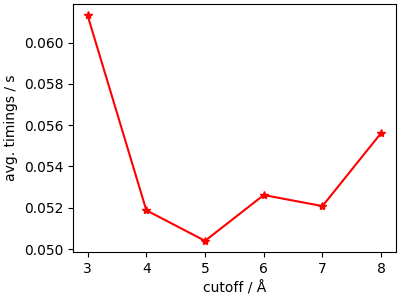
Determining the most efficient cutoff value can be achieved by running a simple search over a few “reasonable” values.

cutoff_grid = torch.tensor([3.0, 4.0, 5.0, 6.0, 7.0, 8.0])

timings_grid = []
for cutoff in cutoff_grid:
    filter_indices, filter_distances = filter_neighbors(
        cutoff, neighbor_indices, neighbor_distances
    )
    smearing, parameters, timing = tune_pme(
        accuracy=1e-5,
        charges=charges,
        cell=cell,
        positions=positions,
        cutoff=cutoff,
        neighbor_indices=filter_indices,
        neighbor_distances=filter_distances,
    )
    timings_grid.append(timing)

/home/runner/work/torch-pme/torch-pme/src/torchpme/tuning/pme.py:265: UserWarning: To copy construct from a tensor, it is recommended to use sourceTensor.clone().detach() or sourceTensor.clone().detach().requires_grad_(True), rather than torch.tensor(sourceTensor).
  cutoff = torch.tensor(cutoff)

Even though the trend is smooth, there is substantial variability, indicating it may be worth to perform this additional tuning whenever the long-range model is the bottleneck of a calculation

fig, ax = plt.subplots(1, 1, figsize=(4, 3), constrained_layout=True)
ax.plot(cutoff_grid, timings_grid, "r-*")
ax.set_ylabel(r"avg. timings / s")
ax.set_xlabel(r"cutoff / Å")

Text(0.5, 18.620124999999987, 'cutoff / Å')