Computing LODE descriptors

Authors:

Michele Ceriotti @ceriottm

This notebook demonstrates the use of some advanced features of torch-pme to compute long-distance equivariants (LODE) features as in Grisafi and Ceriotti, J. Chem. Phys. (2019) and Huguenin-Dumittan et al., J. Phys. Chem. Lett. (2023). Note that a compiled-language CPU implementation of LODE features is also available in the featomic package.

from typing import Optional

import ase
import chemiscope
import matplotlib
import numpy as np
import scipy
import torch
from matplotlib import pyplot as plt

import torchpme
from torchpme.potentials import CoulombPotential, Potential, SplinePotential

device = "cpu"
dtype = torch.float64
rng = torch.Generator()
rng.manual_seed(42)

<torch._C.Generator object at 0x7f8eda7cc390>

Long-distance equivariant descriptors

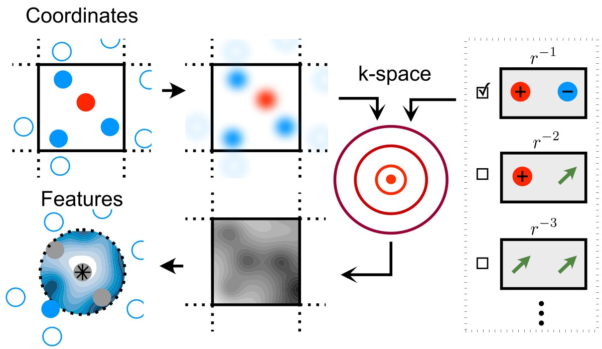
A schematic view of the process of evaluating LODE features. Rather than computing an expansion of the neighbor density (the operation that underlies short-range models, from SOAP to NICE) one first transforms the density in the Fourier domain, then back to obtain a real-space “potential field” that is then expanded on an atom-centered basis.

The basic idea behind the LODE framework is to evaluate a “potential field”, convoluting the neighbor density with a suitable kernel

\[V(\mathbf{x})=\int \mathrm{d}\mathbf{x}' \rho(\mathbf{x}') K(|\mathbf{x}-\mathbf{x}'|)\]

and then expand it on an atom-centered basis, so as to obtain a set of features that describe the environment of each atom.

\[\langle nlm|V_i\rangle =\int \mathrm{d}\mathbf{x}\, V(\mathbf{x}) R_{nl}(x) Y_l^m(\hat{\mathbf{x}})\]

By choosing a slowly-decaying kernel that emphasizes long-range correlations, and that and that is consistent with the asymptotic behavior of e.g. electrostatic interactions, one achieves a description of the long-range interaction, rather than of the immediate vicinity of each atom. By choosing a basis of spherical harmonics for the angular part, one achieves descriptors that transform as irreducible representations of the rotation group.

Initialize a trial structure

We use as an example a distorted rocksalt structure with perturbed positions and charges

structure = ase.Atoms(
    positions=[
        [0, 0, 0],
        [3, 0, 0],
        [0, 3, 0],
        [3, 3, 0],
        [0, 0, 3],
        [3, 0, 3],
        [0, 3, 3],
        [3, 3, 3],
    ],
    cell=[6, 6, 6],
    symbols="NaClClNaClNaNaCl",
)
structure = structure.repeat([3, 3, 3])

displacement = torch.normal(
    mean=0.0, std=2.5e-1, size=(len(structure), 3), generator=rng
)
structure.positions += displacement.numpy()

charges = torch.tensor(
    [[1.0], [-1.0], [-1.0], [1.0], [-1.0], [1.0], [1.0], [-1.0]]
    * (len(structure) // 8),
    dtype=dtype,
    device=device,
).reshape(-1, 1)
charges += torch.normal(mean=0.0, std=1e-1, size=(len(charges), 1), generator=rng)
positions = torch.from_numpy(structure.positions).to(device=device, dtype=dtype)
cell = torch.from_numpy(structure.cell.array).to(device=device, dtype=dtype)

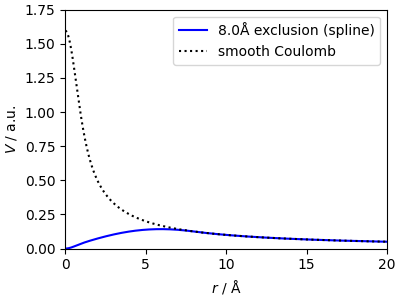
An “excluded-range” smooth Coulomb potential

We use SplinePotential to compute a smooth Coulomb potential with the “short-range” part cut out. This is important as otherwise the potential carries information on the local atomic arrangement, which is redundant (as it is usually described by another part of the model).

CoulombPotential does this by first computing the potential generated by Gaussian densities, and then removing in real space the contributions in the vicinity of each atom. For LODE we must get the potential directly on the grid, and so it is better to use a numerical kernel that achieves this using only k-space operations.

smearing = 0.5
exclusion_radius = 8.0
coulomb = CoulombPotential(smearing=smearing, exclusion_radius=None)
coulomb_exclude = CoulombPotential(smearing=smearing, exclusion_radius=exclusion_radius)

x_grid = torch.logspace(-3, 3, 1000)
y_grid = coulomb_exclude.lr_from_dist(x_grid) + coulomb_exclude.sr_from_dist(x_grid)

# create a spline potential for with the exclusion range built in
spline = SplinePotential(
    r_grid=x_grid, y_grid=y_grid, smearing=smearing, reciprocal=True, yhat_at_zero=0.0
)

t_grid = torch.logspace(-3, 3, 1000)
y_bare = coulomb.lr_from_dist(t_grid)
y_spline = spline.lr_from_dist(t_grid)

fig, ax = plt.subplots(
    1, 1, figsize=(4, 3), sharey=True, sharex=True, constrained_layout=True
)
ax.plot(t_grid, y_spline, "b-", label=f"{exclusion_radius}Å exclusion (spline)")
ax.plot(t_grid, y_bare, "k:", label="smooth Coulomb")

ax.set_xlabel(r"$r$ / Å")
ax.set_ylabel(r"$V$ / a.u.")
ax.set_xlim(0, 20)
ax.set_ylim(0, 1.75)
ax.legend()
fig.show()

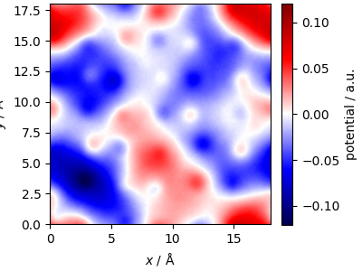
Compute the potential on a mesh

We use MeshInterpolator and KSpaceFilter to compute the potential on a grid.

# Determines grid resolution and initialize utility classes
ns = torchpme.lib.kvectors.get_ns_mesh(cell, smearing * 0.5)
MI = torchpme.lib.MeshInterpolator(
    cell=cell, ns_mesh=ns, interpolation_nodes=3, method="P3M"
)
KF = torchpme.lib.KSpaceFilter(
    cell=cell,
    ns_mesh=ns,
    kernel=spline,
    fft_norm="backward",
    ifft_norm="forward",
)

# Computes particle density on the grid (weighted by the "charges")
MI.compute_weights(positions)
rho_mesh = MI.points_to_mesh(particle_weights=charges)

# Computes the potential using the Fourier filter
ivolume = torch.abs(cell.det()).pow(-1)
potential_mesh = KF(rho_mesh) * ivolume

Plotting a slice of the potential demonstrates the smoothness of the potential, as the “core” region is damped out.

fig, ax = plt.subplots(
    1, 1, figsize=(4, 3), sharey=True, sharex=True, constrained_layout=True
)
mesh_extent = [
    0,
    cell[0, 0],
    0,
    cell[1, 1],
]

z_plot = potential_mesh[0, :, :, 0].cpu().detach().numpy()
z_plot = np.vstack([z_plot, z_plot[0, :]])  # Add first row at the bottom
z_plot = np.hstack(
    [z_plot, z_plot[:, 0].reshape(-1, 1)]
)  # Add first column at the right

z_min, z_max = (z_plot.min(), z_plot.max())
z_range = max(abs(z_min), abs(z_max))

cf = ax.imshow(
    z_plot,
    extent=mesh_extent,
    vmin=-z_range,
    vmax=z_range,
    origin="lower",
    interpolation="bilinear",
    cmap="seismic",
)

ax.set_xlabel(r"$x$ / Å")
ax.set_ylabel(r"$y$ / Å")
fig.colorbar(cf, label=r"potential / a.u.")
fig.show()

Atom-centered grids

To evaluate LODE features, we have to now project the potential within an atom-centered region. To do this, we define an atom-centered grid. Note that the quadrature here is not especially smart, and is only used for demonstrative purposes.

def get_theta_phi_quadrature(L):
    """Legendre quadrature nodes for integrals over theta, phi"""
    quads = []
    weights = []
    for w_index in range(0, 2 * L - 1):
        w = 2 * np.pi * w_index / (2 * L - 1)
        roots_legendre_now, weights_now = scipy.special.roots_legendre(L)
        all_v = np.arccos(roots_legendre_now)
        for v, weight in zip(all_v, weights_now):
            quads.append([v, w])
            weights.append(weight)
    norm = 4 * torch.pi / np.sum(weights)
    return torch.tensor(quads), torch.tensor(weights) * norm


def get_radial_quadrature(order, R):
    """
    Generates Gauss-Legendre quadrature nodes and weights for radial integration
    in spherical coordinates over the interval [0, R].
    """
    gl_nodes, gl_weights = np.polynomial.legendre.leggauss(order)
    nodes = (R / 2) * (gl_nodes + 1)
    weights = (R / 2) ** 3 * gl_weights * (gl_nodes + 1) ** 2

    return torch.from_numpy(nodes), torch.from_numpy(weights)


def get_full_grid(n, R):
    lm_nodes, lm_weights = get_theta_phi_quadrature(n)
    r_nodes, r_weights = get_radial_quadrature(n, R)

    full_weights = (r_weights.reshape(-1, 1) * lm_weights.reshape(1, -1)).flatten()

    cos_nodes = torch.cos(lm_nodes[:, 0]).reshape(1, -1)
    sin_nodes = torch.sin(lm_nodes[:, 0]).reshape(1, -1)
    xyz_nodes = torch.vstack(
        [
            (r_nodes.reshape(-1, 1) * cos_nodes).flatten(),
            (
                r_nodes.reshape(-1, 1) * (sin_nodes * torch.cos(lm_nodes[:, 1]))
            ).flatten(),
            (
                r_nodes.reshape(-1, 1) * (sin_nodes * torch.sin(lm_nodes[:, 1]))
            ).flatten(),
        ]
    ).T

    return xyz_nodes, full_weights


xyz, weights = get_full_grid(3, exclusion_radius / 4)

The grid can then be centered on each atom, and the back-interpolation of MeshInterpolator be used to evaluate the potential values

grid_i = positions[3] + xyz
MI.compute_weights(grid_i)
pots_i = MI.mesh_to_points(potential_mesh).squeeze()

The grid can be shown in the context of the atomic structure

dummy = ase.Atoms(positions=grid_i.numpy(), symbols="H" * len(grid_i))
chemiscope.show(
    frames=[structure + dummy],
    properties={
        "potential": {
            "target": "atom",
            "values": np.concatenate([[0] * len(positions), pots_i.flatten().numpy()]),
        },
        "grid weights": {
            "target": "atom",
            "values": np.concatenate([[0] * len(positions), weights.flatten().numpy()]),
        },
    },
    mode="structure",
    settings=chemiscope.quick_settings(
        structure_settings={
            "unitCell": True,
            "bonds": False,
            "environments": {"activated": False},
            "color": {
                "property": "potential",
                "min": -0.15,
                "max": 0.15,
                "transform": "linear",
                "palette": "seismic",
            },
        }
    ),
    environments=chemiscope.all_atomic_environments([structure + dummy]),
)

×

Computing the projection

In order to compute the LODE coefficients, we simply have to evaluate the basis on the same atom-centered grid. Here for example we just use \((1,x,y,z)\) as basis

# define the basis

f0 = torch.ones(len(xyz))
fx = xyz[:, 0]
fy = xyz[:, 1]
fz = xyz[:, 2]

# normalize the basis

f0 = f0 / torch.sqrt((weights * f0**2).sum())
fx = fx / torch.sqrt((weights * fx**2).sum())
fy = fy / torch.sqrt((weights * fy**2).sum())
fz = fz / torch.sqrt((weights * fz**2).sum())

# compute
lode_i = torch.tensor(
    [
        (weights * f0 * pots_i).sum(),
        (weights * fx * pots_i).sum(),
        (weights * fy * pots_i).sum(),
        (weights * fz * pots_i).sum(),
    ]
).squeeze()

print(f"LODE features: {lode_i}")

LODE features: tensor([-0.4658, -0.0362,  0.0017,  0.0364], dtype=torch.float64)

Defines a LODE calculator

All these pieces can be combined in a relatively concise Calculator class that computes LODE features.

class SmoothCutoffCoulomb(SplinePotential):
    def __init__(
        self, smearing: float, exclusion_radius: float, n_points: Optional[int] = 1000
    ):
        coulomb = CoulombPotential(smearing=smearing, exclusion_radius=exclusion_radius)
        x_grid = torch.logspace(-3, 3, n_points)
        y_grid = coulomb.lr_from_dist(x_grid) + coulomb.sr_from_dist(x_grid)
        super().__init__(
            r_grid=x_grid,
            y_grid=y_grid,
            smearing=smearing,
            exclusion_radius=exclusion_radius,
            reciprocal=True,
            yhat_at_zero=0.0,
        )


class LODECalculator(torchpme.Calculator):
    """
    Compute expansions of the local potential in an atom-centered basis.

    :param potential: A :class:`Potential` implementing the convolution
        kernel. Real-space components are not used.
    :param n_grid: Atom-centered grid size; this is the number of nodes per
        dimension, so the overall number of points is ``n_grid**3``.
    """

    def __init__(self, potential: Potential, n_grid: int = 3):
        super().__init__(potential=potential)

        assert self.potential.exclusion_radius is not None
        assert self.potential.smearing is not None

        cell = torch.eye(3)
        ns = torch.tensor([2, 2, 2])
        self._MI = torchpme.lib.MeshInterpolator(
            cell=cell, ns_mesh=ns, interpolation_nodes=3, method="P3M"
        )
        self._KF = torchpme.lib.KSpaceFilter(
            cell=cell,
            ns_mesh=ns,
            kernel=self.potential,
            fft_norm="backward",
            ifft_norm="forward",
        )

        # assumes a smooth exclusion region so sets the integration cutoff to half that
        nodes, weights = get_full_grid(n_grid, potential.exclusion_radius / 2)

        # these are the "stencils" used to project the potential
        # on an atom-centered basis. NB: weights might also be incorporated
        # in here saving multiplications later on
        stencils = [
            (nodes[:, 0] * 0.0 + 1.0) / torch.sqrt((weights).sum()),  # constant
            (nodes[:, 0]) / torch.sqrt((weights * nodes[:, 0] ** 2).sum()),  # x
            (nodes[:, 1]) / torch.sqrt((weights * nodes[:, 1] ** 2).sum()),  # y
            (nodes[:, 2]) / torch.sqrt((weights * nodes[:, 2] ** 2).sum()),  # z
        ]
        self._basis = torch.stack(stencils)
        self._nodes = nodes
        self._weights = weights

    def forward(
        self,
        charges: torch.Tensor,
        cell: torch.Tensor,
        positions: torch.Tensor,
        neighbor_indices: Optional[torch.Tensor] = None,
        neighbor_distances: Optional[torch.Tensor] = None,
    ) -> torch.Tensor:
        # Update meshes
        assert self.potential.smearing is not None  # otherwise mypy complains
        ns = torchpme.lib.kvectors.get_ns_mesh(cell, self.potential.smearing / 2)
        self._MI.update(cell, ns)
        self._KF.update(cell, ns)

        # Compute potential
        self._MI.compute_weights(positions)
        rho_mesh = self._MI.points_to_mesh(particle_weights=charges)
        ivolume = torch.abs(cell.det()).pow(-1)
        potential_mesh = self._KF(rho_mesh) * ivolume

        # Places integration grids around each atom
        all_points = torch.stack([self._nodes + pos for pos in positions]).reshape(
            -1, 3
        )

        # Evaluate the potential on the grids
        self._MI.compute_weights(all_points)
        all_potentials = self._MI.mesh_to_points(potential_mesh).reshape(
            len(positions), len(self._nodes), -1
        )

        # Compute lode as an integral
        return torch.einsum("ijq,bj,j->ibq", all_potentials, self._basis, self._weights)

Instantiates the calculator and evaluates it for the NaCl structure

smearing = 0.5
exclusion_radius = 8.0
my_pot = SmoothCutoffCoulomb(smearing=smearing, exclusion_radius=exclusion_radius)
my_lode = LODECalculator(potential=my_pot, n_grid=8)

lode_features = my_lode.forward(
    charges=charges, cell=cell, positions=positions
).squeeze()

The basis function hardcoded in the LODECalculator class have a scalar (mean potential) and vectorial (roughly corresponding to the mean electric field) nature, so we can plot it with color corresponding to the constant part, and arrows proportional to the vectorial component.

def value_to_seismic(value, vrange=0.1):
    """Map values to RGB color string using the 'seismic' colormap."""
    vmin, vmax = -vrange, vrange
    # Ensure the value is within the specified range
    clipped_value = np.clip(value, vmin, vmax)
    norm = (clipped_value - vmin) / (vmax - vmin)

    rgba = matplotlib.colormaps["seismic"](norm)
    rgb = tuple(int(255 * c) for c in rgba[:3])
    return "#{:02x}{:02x}{:02x}".format(*rgb)


chemiscope.show(
    frames=[structure],
    properties={
        "lode[1]": {
            "target": "atom",
            "values": np.concatenate([lode_features[:, 0].flatten().numpy()]),
        },
        "lode[x]": {
            "target": "atom",
            "values": np.concatenate([lode_features[:, 1].flatten().numpy()]),
        },
        "lode[y]": {
            "target": "atom",
            "values": np.concatenate([lode_features[:, 2].flatten().numpy()]),
        },
        "lode[z]": {
            "target": "atom",
            "values": np.concatenate([lode_features[:, 3].flatten().numpy()]),
        },
    },
    shapes={
        "lode": {
            "kind": "arrow",
            "parameters": {
                "global": {
                    "baseRadius": 0.2,
                    "headRadius": 0.3,
                    "headLength": 0.5,
                },
                "atom": [
                    {
                        "vector": (4 * lode_features[i, 1:]).tolist(),
                        "color": value_to_seismic(lode_features[i, 0], 0.6),
                    }
                    for i in range(len(lode_features))
                ],
            },
        }
    },
    mode="structure",
    settings=chemiscope.quick_settings(
        structure_settings={
            "unitCell": True,
            "bonds": False,
            "environments": {"activated": False},
            "shape": ["lode"],
        }
    ),
    environments=chemiscope.all_atomic_environments([structure]),
)

×