Examples of the KSpaceFilter class

Authors:

Michele Ceriotti @ceriottm

This notebook demonstrates the use of the KSpaceFilter class to transform a density by applying a scalar filter in reciprocal space.

The class supports many different use cases, and can be reused several times if the filter or the mesh size don’t change.

from time import time

import ase
import chemiscope
import numpy as np
import torch
from matplotlib import pyplot as plt

import torchpme

device = "cpu"
dtype = torch.float64

Demonstrates the application of a k-space filter

We define a fairly rugged function on a mesh, and apply a smoothening filter. We start creating a grid (we use a MeshInterpolator object for simplicity to generate the grid with the right shape) and computing a sharp Gaussian field in the \(xy\) plane.

cell = torch.eye(3, dtype=dtype, device=device) * 6.0
ns_mesh = torch.tensor([9, 9, 9])
interpolator = torchpme.lib.MeshInterpolator(
    cell, ns_mesh, interpolation_nodes=2, method="P3M"
)
xyz_mesh = interpolator.get_mesh_xyz()

mesh_value = (
    np.exp(-4 * ((cell[0, 0] / 2 - xyz_mesh) ** 2)[..., :2].sum(axis=-1))
).reshape(1, *xyz_mesh.shape[:-1])

/home/runner/work/torch-pme/torch-pme/examples/04-kspace-demo.py:49: DeprecationWarning: __array_wrap__ must accept context and return_scalar arguments (positionally) in the future. (Deprecated NumPy 2.0)
  np.exp(-4 * ((cell[0, 0] / 2 - xyz_mesh) ** 2)[..., :2].sum(axis=-1))

To define and apply a Gaussian smearing filter, we first define the convolution kernel that must be applied in the Fourier domain, and then use it as a parameter of the filter class. The application of the filter requires simply a call to lib.KSpaceKernel.compute().

# This is the filter function. NB it is applied
# to the *squared k vector norm*
class GaussianSmearingKernel(torchpme.lib.KSpaceKernel):
    def __init__(self, sigma2: float):
        self._sigma2 = sigma2

    def kernel_from_k_sq(self, k_sq):
        return torch.exp(-k_sq * self._sigma2 * 0.5)


# This is the filter
kernel_filter = torchpme.lib.KSpaceFilter(
    cell, ns_mesh, kernel=GaussianSmearingKernel(sigma2=1.0)
)

# Apply the filter to the mesh
mesh_filtered = kernel_filter.forward(mesh_value)

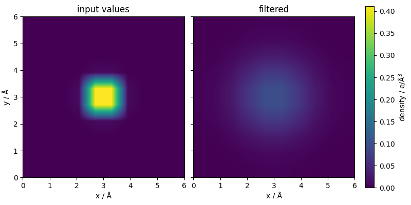
Visualize the effect of the filter

The Gaussian smearing enacted by the filter can be easily visualized taking a slice of the mesh (we make it periodic for a cleaner view)

fig, ax = plt.subplots(
    1, 2, figsize=(8, 4), sharey=True, sharex=True, constrained_layout=True
)
mesh_extent = [
    0,
    cell[0, 0],
    0,
    cell[1, 1],
]

z_plot = mesh_value[0, :, :, 0].detach().numpy()
z_plot = np.vstack([z_plot, z_plot[0, :]])  # Add first row at the bottom
z_plot = np.hstack(
    [z_plot, z_plot[:, 0].reshape(-1, 1)]
)  # Add first column at the right

z_min, z_max = (z_plot.min(), z_plot.max())

cf = ax[0].imshow(
    z_plot,
    extent=mesh_extent,
    vmin=z_min,
    vmax=z_max,
    origin="lower",
    interpolation="bilinear",
)

z_plot = mesh_filtered[0, :, :, 0].detach().numpy()
z_plot = np.vstack([z_plot, z_plot[0, :]])  # Add first row at the bottom
z_plot = np.hstack(
    [z_plot, z_plot[:, 0].reshape(-1, 1)]
)  # Add first column at the right

cf_fine = ax[1].imshow(
    z_plot,
    extent=mesh_extent,
    vmin=z_min,
    vmax=z_max,
    origin="lower",
    interpolation="bilinear",
)
ax[0].set_xlabel("x / Å")
ax[1].set_xlabel("x / Å")
ax[0].set_ylabel("y / Å")
ax[0].set_title(r"input values")
ax[1].set_title(r"filtered")
fig.colorbar(cf_fine, label=r"density / e/Å$^3$")
fig.show()

We can also show the filter in action in 3D, by creating a grid of dummy atoms corresponding to the mesh points, and colored according to the function value. Use the chemiscope option panel to switch between the sharp input and the filtered values.

dummy = ase.Atoms(
    positions=xyz_mesh.reshape(-1, 3),
    symbols="H" * len(xyz_mesh.reshape(-1, 3)),
    cell=cell,
)
chemiscope.show(
    frames=[dummy],
    properties={
        "input value": {
            "target": "atom",
            "values": mesh_value.detach().numpy().flatten(),
        },
        "filtered value": {
            "target": "atom",
            "values": mesh_filtered.detach().numpy().flatten(),
        },
    },
    mode="structure",
    settings=chemiscope.quick_settings(
        structure_settings={
            "unitCell": True,
            "bonds": False,
            "environments": {"activated": False},
            "color": {
                "property": "input value",
                "transform": "linear",
                "palette": "viridis",
            },
        }
    ),
    environments=chemiscope.all_atomic_environments([dummy]),
)

×

Adjustable and multi-channel filters

KSpaceFilter can also be applied for more complicated use cases. For instance, one can apply multiple filters to multiple real-space mesh channels, and use a torch.nn.Module-derived class to define an adjustable kernel.

We initialize a three-channel mesh, with identical patterns along the three Cartesian directions

multi_mesh = torch.stack(
    [
        np.exp(-4 * ((cell[0, 0] / 2 - xyz_mesh) ** 2)[..., :2].sum(axis=-1)),
        np.exp(-4 * ((cell[0, 0] / 2 - xyz_mesh) ** 2)[..., [0, 2]].sum(axis=-1)),
        np.exp(-4 * ((cell[0, 0] / 2 - xyz_mesh) ** 2)[..., 1:].sum(axis=-1)),
    ]
)

/home/runner/work/torch-pme/torch-pme/examples/04-kspace-demo.py:191: DeprecationWarning: __array_wrap__ must accept context and return_scalar arguments (positionally) in the future. (Deprecated NumPy 2.0)
  np.exp(-4 * ((cell[0, 0] / 2 - xyz_mesh) ** 2)[..., :2].sum(axis=-1)),
/home/runner/work/torch-pme/torch-pme/examples/04-kspace-demo.py:192: DeprecationWarning: __array_wrap__ must accept context and return_scalar arguments (positionally) in the future. (Deprecated NumPy 2.0)
  np.exp(-4 * ((cell[0, 0] / 2 - xyz_mesh) ** 2)[..., [0, 2]].sum(axis=-1)),
/home/runner/work/torch-pme/torch-pme/examples/04-kspace-demo.py:193: DeprecationWarning: __array_wrap__ must accept context and return_scalar arguments (positionally) in the future. (Deprecated NumPy 2.0)
  np.exp(-4 * ((cell[0, 0] / 2 - xyz_mesh) ** 2)[..., 1:].sum(axis=-1)),

We also define a filter with three smearing parameters, corresponding to three channels

class MultiKernel(torchpme.lib.KSpaceKernel):
    def __init__(self, sigma: torch.Tensor):
        super().__init__()
        self._sigma = sigma

    def kernel_from_k_sq(self, k_sq):
        return torch.stack([torch.exp(-k_sq * s**2 / 2) for s in self._sigma])

This can be used just as a simple filter

multi_kernel = MultiKernel(torch.tensor([0.25, 0.5, 1.0], dtype=dtype, device=device))
multi_kernel_filter = torchpme.lib.KSpaceFilter(cell, ns_mesh, kernel=multi_kernel)
multi_filtered = multi_kernel_filter.forward(multi_mesh)

When the parameters of the kernel or the cell are modified, one has to call KSpaceFilter.update() before applying the filter

multi_kernel._sigma = torch.tensor([1.0, 0.5, 0.25])
multi_kernel_filter.update(cell)
multi_filtered_2 = multi_kernel_filter.forward(multi_mesh)

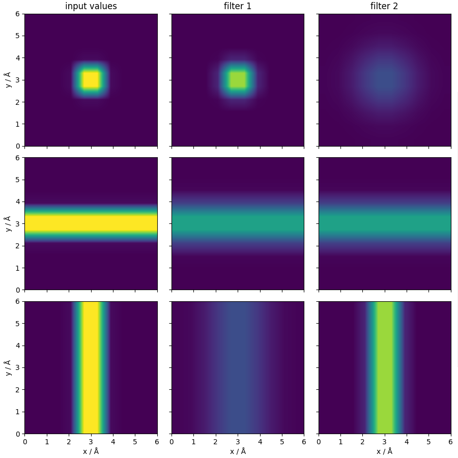
Visualize the application of the filters

The first colum shows the input function (the three channels contain the same function as in the previous example, but with different orientations, which explains the different appearence when sliced along the \(xy\) plane).

The second and third columns show the same three channels with the Gaussian smearings defined above.

fig, ax = plt.subplots(
    3, 3, figsize=(9, 9), sharey=True, sharex=True, constrained_layout=True
)

# reuse the same mesh_extent given the mesh is cubic
mesh_extent = [
    0,
    cell[0, 0],
    0,
    cell[1, 1],
]

z_min, z_max = (mesh_value.flatten().min(), mesh_value.flatten().max())
cfs = []
for j, mesh_value in enumerate([multi_mesh, multi_filtered, multi_filtered_2]):
    for i in range(3):
        z_plot = mesh_value[i, :, :, 4].detach().numpy()
        z_plot = np.vstack([z_plot, z_plot[0, :]])  # Add first row at the bottom
        z_plot = np.hstack(
            [z_plot, z_plot[:, 0].reshape(-1, 1)]
        )  # Add first column at the right

        cf = ax[i, j].imshow(
            z_plot,
            extent=mesh_extent,
            vmin=z_min,
            vmax=z_max,
            origin="lower",
            interpolation="bilinear",
        )
        cfs.append(cf)
    ax[j, 0].set_ylabel("y / Å")
    ax[2, j].set_xlabel("x / Å")

ax[0, 0].set_title("input values")
ax[0, 1].set_title("filter 1")
ax[0, 2].set_title("filter 2")
cbar_ax = fig.add_axes(
    [1.0, 0.2, 0.03, 0.6]
)  # [left, bottom, width, height] in figure coordinates
# Add the colorbar to the new axes
fig.colorbar(cfs[0], cax=cbar_ax, orientation="vertical")

<matplotlib.colorbar.Colorbar object at 0x7f8efb447c50>

Jit-ting of the k-space filter

The k-space filter can also be compiled to torch-script, for faster execution (the impact is marginal for this very simple case)

multi_filtered = multi_kernel_filter.forward(multi_mesh)
start = time()
for _i in range(100):
    multi_filtered = multi_kernel_filter.forward(multi_mesh)
time_python = (time() - start) * 1e6 / 100

jitted_kernel_filter = torch.jit.script(multi_kernel_filter)
jit_filtered = jitted_kernel_filter.forward(multi_mesh)
start = time()
for _i in range(100):
    jit_filtered = jitted_kernel_filter.forward(multi_mesh)
time_jit = (time() - start) * 1e6 / 100

print(f"Evaluation time:\nPytorch: {time_python}µs\nJitted:  {time_jit}µs")

Evaluation time:
Pytorch: 77.28815078735352µs
Jitted:  92.61608123779297µs