Examples of the MeshInterpolator class

Authors:

Michele Ceriotti @ceriottm

This notebook showcases the functionality of torch-pme by going step-by-step through the process of projecting an atom density onto a grid, and interpolating the grid values on (possibly different) points.

import ase
import chemiscope
import numpy as np
import torch
from matplotlib import pyplot as plt

import torchpme

device = "cpu"
dtype = torch.float64
rng = torch.Generator()
rng.manual_seed(32)

<torch._C.Generator object at 0x7f8eecb48030>

Compute the atom density projection on a mesh

Create a rocksalt structure with a regular array of atoms, that we will use as example

structure = ase.Atoms(
    positions=[
        [0, 0, 0],
        [3, 0, 0],
        [0, 3, 0],
        [3, 3, 0],
        [0, 0, 3],
        [3, 0, 3],
        [0, 3, 3],
        [3, 3, 3],
    ],
    cell=[6, 6, 6],
    symbols="NaClClNaClNaNaCl",
)

We now slightly displace the atoms from their initial positions randomly based on a Gaussian distribution.

displacement = torch.normal(
    mean=0.0, std=2.5e-1, size=(len(structure), 3), generator=rng
)
structure.positions += displacement.numpy()

chemiscope.show(
    frames=[structure],
    mode="structure",
    settings=chemiscope.quick_settings(structure_settings={"unitCell": True}),
)

×

We also define the charges, with a bit of noise for good measure. (NB: the structure won’t be charge neutral but it does not matter for this example). Also load positions and cells into torch tensors

charges = torch.tensor(
    [[1.0], [-1.0], [-1.0], [1.0], [-1.0], [1.0], [1.0], [-1.0]],
    dtype=dtype,
    device=device,
)
charges += torch.normal(mean=0.0, std=1e-1, size=(len(charges), 1), generator=rng)
positions = torch.from_numpy(structure.positions).to(device=device, dtype=dtype)
cell = torch.from_numpy(structure.cell.array).to(device=device, dtype=dtype)

We now use MeshInterpolator to project atomic positions on a grid. Note that ideally the interpolation represents a sharp density peaked at atomic positions, so the degree of smoothening depends on the grid resolution (as well as on the interpolation nodes)

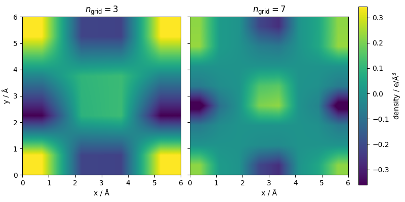
We demonstrate this by computing a projection on two grids with 3 and 7 mesh points.

interpolator = torchpme.lib.MeshInterpolator(
    cell=cell, ns_mesh=torch.tensor([3, 3, 3]), interpolation_nodes=3, method="P3M"
)
interpolator_fine = torchpme.lib.MeshInterpolator(
    cell=cell, ns_mesh=torch.tensor([7, 7, 7]), interpolation_nodes=3, method="P3M"
)
interpolator.compute_weights(positions)
interpolator_fine.compute_weights(positions)

rho_mesh = interpolator.points_to_mesh(charges)
rho_mesh_fine = interpolator_fine.points_to_mesh(charges)

Note that the meshing can be also used for multiple “pseudo-charge” values per atom simultaneously. In that case, points_to_mesh will return multiple mesh values.

pseudo_charges = torch.normal(mean=0, std=1, size=(len(structure), 4))
pseudo_mesh = interpolator.points_to_mesh(pseudo_charges)

print(tuple(pseudo_mesh.shape))

(4, 3, 3, 3)

Visualizing the mesh

One can extract the mesh to visualize the values of the atom density. The grid is periodic, so we need some manipulations just for the purpose of visualization. It is clear that the finer mesh leads to sharper densities, centered around the atom positions.

fig, ax = plt.subplots(
    1, 2, figsize=(8, 4), sharey=True, sharex=True, constrained_layout=True
)
mesh_extent = [
    0,
    interpolator.cell[0, 0],
    0,
    interpolator.cell[1, 1],
]

z_plot = rho_mesh[0, :, :, 0].detach().numpy()
z_plot = np.vstack([z_plot, z_plot[0, :]])  # Add first row at the bottom
z_plot = np.hstack(
    [z_plot, z_plot[:, 0].reshape(-1, 1)]
)  # Add first column at the right

z_min, z_max = (z_plot.min(), z_plot.max())

cf = ax[0].imshow(
    z_plot,
    extent=mesh_extent,
    vmin=z_min,
    vmax=z_max,
    origin="lower",
    interpolation="bilinear",
)

z_plot = rho_mesh_fine[0, :, :, 0].detach().numpy()
z_plot = np.vstack([z_plot, z_plot[0, :]])  # Add first row at the bottom
z_plot = np.hstack(
    [z_plot, z_plot[:, 0].reshape(-1, 1)]
)  # Add first column at the right

cf_fine = ax[1].imshow(
    z_plot,
    extent=mesh_extent,
    vmin=z_min,
    vmax=z_max,
    origin="lower",
    interpolation="bilinear",
)
ax[0].set_xlabel("x / Å")
ax[1].set_xlabel("x / Å")
ax[0].set_ylabel("y / Å")
ax[0].set_title(r"$n_{\mathrm{grid}}=3$")
ax[1].set_title(r"$n_{\mathrm{grid}}=7$")
fig.colorbar(cf_fine, label=r"density / e/Å$^3$")
fig.show()

Mesh visualization in chemiscope

We can also plot the points explicitly together with the structure, adding some dummy atoms with a “charge” property

xyz_mesh = interpolator.get_mesh_xyz().detach().numpy()
dummy = ase.Atoms(
    positions=xyz_mesh.reshape(-1, 3), symbols="H" * len(xyz_mesh.reshape(-1, 3))
)
chemiscope.show(
    frames=[structure + dummy],
    properties={
        "charge": {
            "target": "atom",
            "values": np.concatenate([charges.flatten(), rho_mesh[0].flatten()]),
        }
    },
    mode="structure",
    settings=chemiscope.quick_settings(
        structure_settings={
            "unitCell": True,
            "bonds": False,
            "environments": {"activated": False},
            "color": {
                "property": "charge",
                "min": -0.3,
                "max": 0.3,
                "transform": "linear",
                "palette": "seismic",
            },
        }
    ),
    environments=chemiscope.all_atomic_environments([structure + dummy]),
)

×

and for the fine mesh (that again shows clearly how the charge is distributed over the neighboring points, and how the mesh size determines the smearing).

xyz_mesh = interpolator_fine.get_mesh_xyz().detach().numpy()
dummy = ase.Atoms(
    positions=xyz_mesh.reshape(-1, 3), symbols="H" * len(xyz_mesh.reshape(-1, 3))
)
chemiscope.show(
    frames=[structure + dummy],
    properties={
        "charge": {
            "target": "atom",
            "values": np.concatenate([charges.flatten(), rho_mesh_fine[0].flatten()]),
        }
    },
    mode="structure",
    settings=chemiscope.quick_settings(
        structure_settings={
            "unitCell": True,
            "bonds": False,
            "environments": {"activated": False},
            "color": {
                "property": "charge",
                "min": -0.3,
                "max": 0.3,
                "transform": "linear",
                "palette": "seismic",
            },
        }
    ),
    environments=chemiscope.all_atomic_environments([structure + dummy]),
)

×

Mesh interpolation

Once a mesh has been defined, it is possible to use the MeshInterpolator object to compute an interpolation of the field on the points for which the weights have been computed.

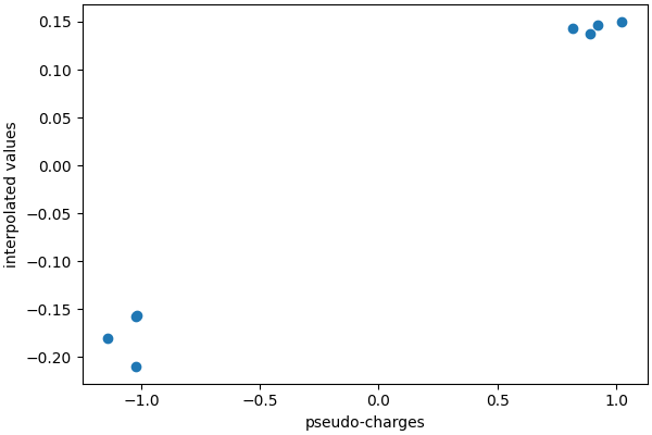
A very important point to grasp is that the charge mapping on the grid is designed to conserve the total charge, and so interpolating it back does not (and is not meant to!) yield the initial value of the atomic “pseudo-charges”.

This is also very clear from the mesh plots above, in which the charge assigned to the grid points is much smaller than the atomic charges (that are around ±1).

mesh_charges = interpolator_fine.mesh_to_points(rho_mesh_fine)
fig, ax = plt.subplots(1, 1, figsize=(6, 4), constrained_layout=True)

ax.scatter(charges.flatten(), mesh_charges.flatten())
ax.set_xlabel("pseudo-charges")
ax.set_ylabel("interpolated values")
fig.show()

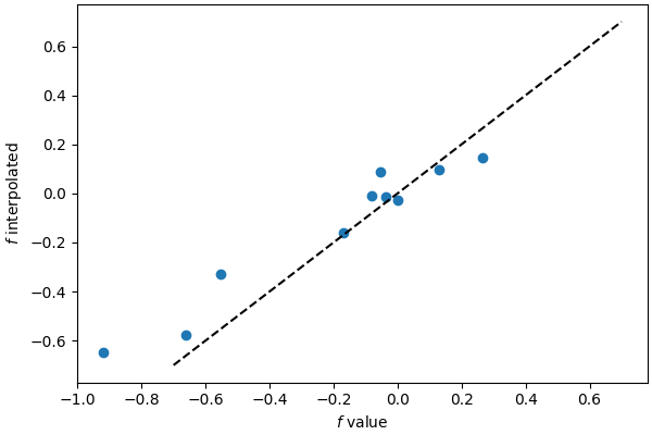
Even though it is not specifically designed for that, points_to_mesh can interpolate arbitrary functions defined on the grid. For instance, here we define a product of sine functions along the three Cartesian directions, \(\cos(2\pi x/L)\cos(2\pi y/L)\cos(2\pi z/L)\)

xyz_mesh = interpolator_fine.get_mesh_xyz()
mesh_2pil = xyz_mesh * np.pi * 2 / interpolator_fine.cell[0, 0]
f_mesh = (
    torch.cos(mesh_2pil[..., 0])
    * torch.cos(mesh_2pil[..., 1])
    * torch.cos(mesh_2pil[..., 2])
).reshape(1, *mesh_2pil.shape[:-1])

f_points = interpolator_fine.mesh_to_points(f_mesh)

dummy = ase.Atoms(
    positions=xyz_mesh.reshape(-1, 3), symbols="H" * len(xyz_mesh.reshape(-1, 3))
)
chemiscope.show(
    frames=[structure + dummy],
    properties={
        "f": {
            "target": "atom",
            "values": np.concatenate([f_points.flatten(), f_mesh.flatten()]),
        }
    },
    mode="structure",
    settings=chemiscope.quick_settings(
        structure_settings={
            "unitCell": True,
            "bonds": False,
            "environments": {"activated": False},
            "color": {
                "property": "f",
                "min": -1,
                "max": 1,
                "transform": "linear",
                "palette": "seismic",
            },
        }
    ),
    environments=chemiscope.all_atomic_environments([structure + dummy]),
)

×

Interpolating on different points

If you want to interpolate on a different set of points than the ones a MeshInterpolator object was initialized on, it is easy to do by either creating a new one or simply calling again compute_weights for the new set of points.

new_points = torch.normal(mean=3, std=1, size=(10, 3), dtype=dtype, device=device)
interpolator_fine.compute_weights(new_points)
new_f = interpolator_fine.mesh_to_points(f_mesh)
new_ref = (
    torch.cos(new_points[..., 0])
    * torch.cos(new_points[..., 1])
    * torch.cos(new_points[..., 2])
).reshape(1, *new_points.shape[:-1])

Even though the interpolated values are not accurate (this is a pretty coarse grid for this function resolution) it is clear that the class can interpolate on arbitrary positions of the target points.

fig, ax = plt.subplots(1, 1, figsize=(6, 4), constrained_layout=True)

ax.scatter(new_ref.flatten(), new_f.flatten())
ax.plot([-0.7, 0.7], [-0.7, 0.7], "k--")
ax.set_xlabel(r"$f$ value")
ax.set_ylabel(r"$f$ interpolated")
fig.show()