Atomistic model for molecular dynamics

In this example, we demonstrate how to construct a metatensor atomistic model based on the metatensor interface of torchpme. The model will be used to run a very short molecular dynamics (MD) simulation of a non-neutral hydroden plasma in a cubic box. The plasma consists of massive point particles which are interacting pairwise via a Coulomb force which we compute using the EwaldCalculator.

The tutorial assumes knowledge of torchpme and how to export an metatensor atomistic model to run it with the ASE calculator. For learning these details we refer to the metatensor atomistic tutorials.

from typing import Dict, List, Optional  # noqa

# tools to run the simulation and visualization
import ase.md
import ase.visualize.plot
import ase.md.velocitydistribution
import chemiscope
import metatensor.torch
import matplotlib.pyplot as plt

# tools to wrap and run the model
import numpy as np
import torch
from metatensor.torch import Labels, TensorBlock, TensorMap
from metatensor.torch.atomistic import (
    MetatensorAtomisticModel,
    ModelCapabilities,
    ModelEvaluationOptions,
    ModelMetadata,
    ModelOutput,
    NeighborListOptions,
    System,
)

# Integration with ASE calculator for metatensor atomistic models
from metatensor.torch.atomistic.ase_calculator import MetatensorCalculator

# the usual suspect
import torchpme

The simulation system

Create a system of 12 hydrogen atoms in a cubic periodic box of \(10\,\text{Å}\) side length.

rng = np.random.default_rng(42)
atoms = ase.Atoms(
    12 * "H",
    positions=10 * rng.random([12, 3]),
    cell=10 * np.eye(3),
    pbc=True,
)

We now can visualize the system with chemiscope.

chemiscope.show(
    [atoms],
    mode="structure",
    settings=chemiscope.quick_settings(
        trajectory=True, structure_settings={"unitCell": True}
    ),
)

×

Assigning charges

For computing the electrostatic potential we need to assign charges to a metatensor.torch.atomistic.System since charges will not be provided by the engine. Here, we define a simple charge assignment scheme based on the atomic number. We set the partial charge of all hydrogens \(1\) in terms of the elementary charge. Such an assignemnt scheme can also be more complex and for example deduce the charges from a short range machine learning model.

def add_charges(system: System) -> None:
    dtype = system.positions.dtype
    device = system.positions.device

    # set charges of all atoms to 1
    charges = torch.ones(len(system), 1, dtype=dtype, device=device)

    # Create metadata for the charges TensorBlock
    samples = Labels("atom", torch.arange(len(system), device=device).reshape(-1, 1))
    properties = Labels("charge", torch.zeros(1, 1, device=device, dtype=torch.int32))
    block = TensorBlock(
        values=charges, samples=samples, components=[], properties=properties
    )

    tensor = TensorMap(
        keys=Labels("_", torch.zeros(1, 1, dtype=torch.int32)), blocks=[block]
    )

    system.add_data(name="charges", tensor=tensor)

Warning

Having non-charge neutral system is not problematic for this simulation. Even though any Ewald method requires a charge-neutral system, charged system will be neutralized by adding an homogenous background density. This background charge adds an additional contribution to the real-space interaction which is already accountaed for by torchpme. For homogenous and isotropic systems a nonzero background charge will not have an effect on the simulation but it will for inhomgenous system. For more information see e.g. Hub et.al.

We now test the assignmenet by creating a test system and adding the charges.

system = System(
    types=torch.from_numpy(atoms.get_atomic_numbers()),
    positions=torch.from_numpy(atoms.positions),
    cell=torch.from_numpy(atoms.cell.array),
    pbc=torch.from_numpy(atoms.pbc),
)

add_charges(system)

print(system.get_data("charges").block().values)

tensor([[1.],
        [1.],
        [1.],
        [1.],
        [1.],
        [1.],
        [1.],
        [1.],
        [1.],
        [1.],
        [1.],
        [1.]], dtype=torch.float64)

As expected the charges are assigned to all atoms based on their atomic number.

The model

We now define the atomistic model that computes the potential based on a given calculator and the cutoff. The cutoff is required to define the neighbor list which will be used to compute the short range part of the potential. The design of the model is inspire by the Lennard-Jones model.

Inside the forward method we compute the potential at the atomci positions, which is then multiplied by the formal “charges” to obtain a per-atom energy.

class CalculatorModel(torch.nn.Module):
    def __init__(self, calculator: torchpme.metatensor.Calculator, cutoff: float):
        super().__init__()

        self.calculator = calculator

        # We use a half neighborlist and allow to have pairs farther than cutoff
        # (`strict=False`) since this is not problematic for PME and may speed up the
        # computation of the neigbors.
        self.nl = NeighborListOptions(cutoff=cutoff, full_list=False, strict=False)

    def requested_neighbor_lists(self):
        return [self.nl]

    def _setup_systems(
        self,
        systems: list[System],
        selected_atoms: Optional[Labels] = None,
    ) -> tuple[System, TensorBlock]:
        """Remove possible ghost atoms and add charges to the system."""
        if len(systems) > 1:
            raise ValueError(f"only one system supported, got {len(systems)}")

        system_i = 0
        system = systems[system_i]

        # select only real atoms and discard ghosts
        if selected_atoms is not None:
            current_system_mask = selected_atoms.column("system") == system_i
            current_atoms = selected_atoms.column("atom")
            current_atoms = current_atoms[current_system_mask].to(torch.long)

            types = system.types[current_atoms]
            positions = system.positions[current_atoms]
        else:
            types = system.types
            positions = system.positions

        system_final = System(types, positions, system.cell, system.pbc)
        add_charges(system_final)

        return system_final, system.get_neighbor_list(self.nl)

    def forward(
        self,
        systems: List[System],  # noqa
        outputs: Dict[str, ModelOutput],  # noqa
        selected_atoms: Optional[Labels] = None,
    ) -> Dict[str, TensorMap]:  # noqa
        if list(outputs.keys()) != ["energy"]:
            raise ValueError(
                f"`outputs` keys ({', '.join(outputs.keys())}) contain unsupported "
                "keys. Only 'energy' is supported."
            )

        system, neighbors = self._setup_systems(systems, selected_atoms)

        # compute the potential using torchpme
        potential = self.calculator.forward(system, neighbors)

        # Create a reference charge block with the same metadata as the potential to
        # allow multiplcation which requries same metadata
        charges_block = TensorBlock(
            values=system.get_data("charges").block().values,
            samples=potential[0].samples,
            components=potential[0].components,
            properties=potential[0].properties,
        )
        charge_map = TensorMap(keys=potential.keys, blocks=[charges_block])
        energy_per_atom = metatensor.torch.multiply(potential, charge_map)

        if outputs["energy"].per_atom:
            energy = energy_per_atom
        else:
            energy = metatensor.torch.sum_over_samples(
                energy_per_atom, sample_names="atom"
            )

        # Rename property label to follow metatensor's covention for an atomistic model
        old_block = energy[0]
        block = TensorBlock(
            values=old_block.values,
            samples=old_block.samples,
            components=old_block.components,
            properties=old_block.properties.rename("charges_channel", "energy"),
        )

        return {"energy": TensorMap(keys=energy.keys, blocks=[block])}

Warning

Due to limitatations in the engine interface of the MetatensorAtomisticModel, the evaluation of the energy for a subset of atoms is not supported. If you want to compute the energy for a subset you have to filter the contributions after the computation of the whole system.

Define a calculator

To test the model we need to define a calculator that computes the potential. We here use a the metatensor.EwaldCalculator and a CoulombPotential.

Note

We here use the Ewald method and PME because the system only contains 16 atoms. For such small systems the Ewald method is up to 6 times faster compared to PME. If your system reaches a size of 1000 atoms it is recommended to use metatensor.PMECalculator, or metatensor.P3MCalculator that implements the particle-particle/particle-mesh method. See at the end of this tutorial for an example.

These are rather tight settings you can try tune_ewald to determine automatically parameters with a target accuracy

smearing, ewald_params, cutoff = 8.0, {"lr_wavelength": 64.0}, 32.0

We now define an Ewald calculator with a Coulomb potential.

calculator = torchpme.metatensor.EwaldCalculator(
    torchpme.CoulombPotential(smearing=smearing),
    **ewald_params,
    prefactor=torchpme.prefactors.eV_A,
)

Define model metatdata

We now initilize the model and wrap it in a metatensor atomistic model defining all necessary metatdata.

This contains the (energy) units and length units.

energy_unit = "eV"
length_unit = "angstrom"

We now have to define what our model is able to compute. The metatensor.torch.atomistic.ModelOutput defines that the model will compute the energy in eV. Besides the obvous parameters (atomic_types, supported_devices and the dtype) it is very important to set interaction_range to be infinite. For a finite range the provided system of the engine might only contain a subset of the system which will lead to wrong results!

outputs = {"energy": ModelOutput(quantity="energy", unit=energy_unit, per_atom=False)}
options = ModelEvaluationOptions(
    length_unit=length_unit, outputs=outputs, selected_atoms=None
)

model_capabilities = ModelCapabilities(
    outputs=outputs,
    atomic_types=[1],
    interaction_range=torch.inf,
    length_unit=length_unit,
    supported_devices=["cpu", "cuda"],
    dtype="float32",
)

Initilize and wrap the model

model = CalculatorModel(calculator=calculator, cutoff=cutoff)
model.eval()

atomistic_model = MetatensorAtomisticModel(
    model.eval(), ModelMetadata(), model_capabilities
)

We’ll run the simulation in the constant volume/temperature thermodynamic ensemble (NVT or Canonical ensemble), using a Langevin thermostat for time integration. Please refer to the corresponding documentation (ase.md.langevin.Langevin) for more information!

To start the simulation we first set the atomistic_model as the calculator for our plasma.

ewald_mta_calculator = MetatensorCalculator(atomistic_model)
atoms.calc = ewald_mta_calculator

Set initial velocities according to the Maxwell-Boltzmann distribution

ase.md.velocitydistribution.MaxwellBoltzmannDistribution(atoms, 10_000 * ase.units.kB)

/home/runner/work/torch-pme/torch-pme/.tox/docs/lib/python3.13/site-packages/ase/md/md.py:52: FutureWarning: Specify the temperature in K using the 'temperature_K' argument
  warnings.warn(FutureWarning(w))

Set up the Langevin thermostat for NVT ensemble

integrator = ase.md.Langevin(
    atoms,
    timestep=2 * ase.units.fs,
    temperature_K=10_000,
    friction=0.1 / ase.units.fs,
)

Run the simulation

We now have everything in place run the simulation for 50 steps (\(2\,\mathrm{fs}\)) and collect the potential, kinetic and total energy as well as the temperature and pressure.

n_steps = 500

potential_energy = np.zeros(n_steps)
kinetic_energy = np.zeros(n_steps)
total_energy = np.zeros(n_steps)
temperature = np.zeros(n_steps)
pressure = np.zeros(n_steps)
trajectory = []

for i_step in range(n_steps):
    integrator.run(1)

    # collect data about the simulation
    trajectory.append(atoms.copy())
    potential_energy[i_step] = atoms.get_potential_energy()
    kinetic_energy[i_step] = atoms.get_kinetic_energy()
    total_energy[i_step] = atoms.get_total_energy()
    temperature[i_step] = atoms.get_temperature()
    pressure[i_step] = -np.diagonal(atoms.get_stress(voigt=False)).mean()

We can now use chemiscope to visualize the trajectory. For better visualization we wrap the atoms inside the unit cell.

for atoms in trajectory:
    atoms.wrap()

chemiscope.show(
    trajectory,
    mode="structure",
    settings=chemiscope.quick_settings(
        trajectory=True, structure_settings={"unitCell": True}
    ),
)

×

Analyze the results

And look at the time evolution of some physical constants for our system

fig, ax = plt.subplots(3, figsize=(8, 5), sharex=True)

time = 2.0 * np.arange(n_steps)

ax[0].plot(time, potential_energy, label="potential energy")
ax[0].plot(time, kinetic_energy, label="kinetic energy")
ax[0].plot(time, total_energy, label="total energy")
ax[0].legend(ncol=3)
ax[0].set_ylabel("energy [eV]")

ax[1].plot(time, temperature, label="temperature")
ax[1].axhline(10_000, color="black", linestyle="--", label="target temperature")
ax[1].legend(ncol=2)
ax[1].set_ylabel("temperature [K]")

ax[2].plot(time, pressure)
ax[2].set_ylabel("pressure [eV Å$^{-3}$]")

ax[-1].set_xlabel("time / fs")

fig.align_labels()
plt.show()

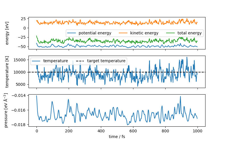
Given the presence of a Langevin thermostat, the total energy is not conserved, but the temperature is well-controlled and fluctuates around the target value of 10,000 K. The metatensor interface also is able to compute the pressure of the simulation via auto differentiation, which is plotted as well. If you want to know more about thermostats and constant-temperature molecular dynamics, you can see this tutorial.

This atomistic model can also be used in other engines like LAMMPS. See the metatensor atomistic page on supported simulation engines. The presented model can also be used in more complex sitatuations, e.g. to compute only the electrostatic potential while other parts of the simulations such as the Lennard-Jones potential are computed by other calculators inside the simulation engine.

A comparison between calculators

Even though, as discussed above, for such a small simulation the Ewald method is likely to be the most efficient, it is easy to set up a model that uses the PME, or P3M, calculators in torchpme. For example,

# PME
smearing, ewald_params, cutoff = (
    0.5,
    {"mesh_spacing": 0.25, "interpolation_nodes": 4},
    8.0,
)

pme_calculator = torchpme.metatensor.PMECalculator(
    torchpme.CoulombPotential(smearing=smearing),
    **ewald_params,
    prefactor=torchpme.prefactors.eV_A,
)

pme_model = CalculatorModel(calculator=pme_calculator, cutoff=cutoff)

pme_atomistic_model = MetatensorAtomisticModel(
    pme_model.eval(), ModelMetadata(), model_capabilities
)

pme_mta_calculator = MetatensorCalculator(pme_atomistic_model)

# P3M
p3m_calculator = torchpme.metatensor.P3MCalculator(
    torchpme.CoulombPotential(smearing=smearing),
    **ewald_params,
    prefactor=torchpme.prefactors.eV_A,
)

p3m_model = CalculatorModel(calculator=p3m_calculator, cutoff=cutoff)

p3m_atomistic_model = MetatensorAtomisticModel(
    p3m_model.eval(), ModelMetadata(), model_capabilities
)

p3m_mta_calculator = MetatensorCalculator(p3m_atomistic_model)

We can then compare the values obtained with the two Ewald engines

# gets the energy from the Ewald calculator
atoms.calc = ewald_mta_calculator
ewald_energy = atoms.get_potential_energy()
ewald_forces = atoms.get_forces()

# overrides the calculator and computes PME
atoms = atoms.copy()
atoms.calc = pme_mta_calculator
pme_energy = atoms.get_potential_energy()
pme_forces = atoms.get_forces()

# ... and P3M
atoms = atoms.copy()
atoms.calc = p3m_mta_calculator
p3m_energy = atoms.get_potential_energy()
p3m_forces = atoms.get_forces()

print(
    f"Energy (Ewald): {ewald_energy}\n"
    f"Energy (PME):   {pme_energy}\n"
    f"Energy (P3M):   {p3m_energy}\n"
)
print(
    f"Forces (Ewald):\n{ewald_forces}\n\n"
    f"Forces (PME):\n{pme_forces}\n\n"
    f"Forces (P3M):\n{p3m_forces}"
)

Energy (Ewald): -50.571353912353516
Energy (PME):   -50.52611541748047
Energy (P3M):   -50.52189254760742

Forces (Ewald):
[[ 0.09059066  0.44978419 -0.90444809]
 [-0.37997434 -2.0111928   1.07122648]
 [ 0.18100952 -0.43447021 -0.03110215]
 [ 1.462111    1.1936059   0.03581454]
 [-0.85438287 -0.05459023  0.40494722]
 [-0.17709282 -0.473171   -0.11635519]
 [-0.41979057  0.39633575 -0.47465798]
 [-0.05026046 -0.53184015 -0.22202076]
 [ 0.34676024  0.19488281  0.14477026]
 [ 0.74841189  0.34315687  0.49568146]
 [ 1.20114195  1.10904992 -0.30248025]
 [-2.14852881 -0.18155357 -0.10137586]]

Forces (PME):
[[ 0.09481248  0.44857794 -0.90494817]
 [-0.38760597 -2.00512981  1.07789755]
 [ 0.1772218  -0.44207641 -0.03918238]
 [ 1.45665932  1.18973684  0.03450844]
 [-0.84592515 -0.05447095  0.40587896]
 [-0.17136928 -0.46527734 -0.11410771]
 [-0.42817628  0.38999006 -0.4783752 ]
 [-0.0519303  -0.52337688 -0.21536151]
 [ 0.3421914   0.2006797   0.1378473 ]
 [ 0.75634819  0.34439543  0.49703431]
 [ 1.20872116  1.10101509 -0.30976978]
 [-2.14461827 -0.1839259  -0.09277071]]

Forces (P3M):
[[ 0.09129928  0.44955575 -0.90452892]
 [-0.38069603 -2.01033592  1.07196772]
 [ 0.18033987 -0.43509534 -0.03153744]
 [ 1.46141398  1.19291496  0.03553772]
 [-0.85430956 -0.05454677  0.40515703]
 [-0.17627423 -0.4728452  -0.11593961]
 [-0.42024806  0.39555588 -0.47535861]
 [-0.05051793 -0.53170562 -0.22120857]
 [ 0.34617156  0.19568491  0.14406092]
 [ 0.74886841  0.3434746   0.4960297 ]
 [ 1.2017554   1.1085912  -0.30324963]
 [-2.14785647 -0.181995   -0.10121254]]

The above output shows us that these values are very close to each other, as expected.