Splined potentials

Authors:

Michele Ceriotti @ceriottm

This notebook demonstrates the use of the SplinePotential class to evaluate potentials for which there is no simple analytical expression for the Fourier-domain filter.

import ase
import numpy as np
import torch
from matplotlib import pyplot as plt

import torchpme
from torchpme.potentials import CoulombPotential, SplinePotential

device = "cpu"
dtype = torch.float64
rng = torch.Generator()
rng.manual_seed(42)

<torch._C.Generator object at 0x7f8fb059c2d0>

Defining the potential on a radial grid

The SplinePotential can be initialized using simply a pair of arrays: radial positions, and the corresponding values of the potential

x_grid = torch.linspace(0, 10, 8, device=device, dtype=dtype)
y_grid = torch.exp(-(x_grid**2) / 2) / torch.pow(torch.pi * 2, torch.tensor([3 / 2]))

x_grid_fine = torch.linspace(0, 10, 32, device=device, dtype=dtype)
y_grid_fine = torch.exp(-(x_grid_fine**2) / 2) / torch.pow(
    torch.pi * 2, torch.tensor([3 / 2])
)

spline = SplinePotential(r_grid=x_grid, y_grid=y_grid)
spline_fine = SplinePotential(r_grid=x_grid_fine, y_grid=y_grid_fine)

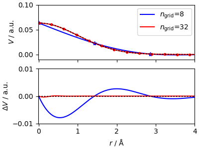
The real-space function can be easily evaluated using the lr_from_dist member function. The convergence with number of spline points is fast, for such a slowly-varying function.

x_test = torch.linspace(0, 10, 256, device=device, dtype=dtype)
y_test = torch.exp(-(x_test**2) / 2) / torch.pow(torch.pi * 2, torch.tensor([3 / 2]))
y_spline = spline.lr_from_dist(x_test)
y_spline_fine = spline_fine.lr_from_dist(x_test)

fig, ax = plt.subplots(2, 1, figsize=(4, 3), sharex=True, constrained_layout=True)

ax[0].plot(x_grid, y_grid, "b*")
ax[0].plot(x_test, y_spline, "b-", label=r"$n_\mathrm{grid}$=8")
ax[0].plot(x_grid_fine, y_grid_fine, "r.")
ax[0].plot(x_test, y_spline_fine, "r-", label=r"$n_\mathrm{grid}$=32")
ax[0].plot(x_test, y_test, "k:")
ax[1].set_xlabel(r"$r$ / Å")
ax[0].set_ylabel(r"$V$ / a.u.")
ax[0].set_xlim(-0.01, 4)
ax[0].set_ylim(-0.01, 0.1)

ax[1].set_ylabel(r"$\Delta V$ / a.u.")
ax[1].plot(x_test, y_spline - y_test, "b-")
ax[1].plot(x_test, y_spline_fine - y_test, "r-")
ax[1].plot(x_test, y_test * 0, "k:")
ax[1].set_ylim(-1e-2, 1e-2)
ax[0].legend()

<matplotlib.legend.Legend object at 0x7f8edaf2e850>

Fourier-domain kernel

A core feature of SplinePotential is that it can evaluate automatically the Fourier-domain kernel that is used in k-space methods. This is done by evaluating

\[\hat{f}(k) =4\pi\int \mathrm{d}r \frac{\sin k r}{k} r f(r)\]

in a semin-analytical way - that is, by computing the integral over each segment in the cubic spline.

k_test = torch.linspace(0, 10, 256, device=device, dtype=dtype)
yhat_test = torch.exp(-(k_test**2) / 2)  # /torch.pow(2*torch.pi,torch.tensor([3/2]))

yhat_spline = spline.kernel_from_k_sq(k_test**2)
yhat_spline_fine = spline_fine.kernel_from_k_sq(k_test**2)

fig, ax = plt.subplots(1, 1, figsize=(4, 3), sharex=True, constrained_layout=True)

ax.plot(x_test, yhat_spline, "b-", label=r"$n_\mathrm{grid}$=8")
ax.plot(x_test, yhat_spline_fine, "r-", label=r"$n_\mathrm{grid}$=32")
ax.plot(k_test, yhat_test, "k:")
ax.set_xlabel(r"$k$ / Å$^{-1}$")
ax.set_ylabel(r"$\hat{V}$ / a.u.")
ax.set_xlim(-0.01, 4)
ax.set_ylim(-0.1, 1.1)
ax.legend()

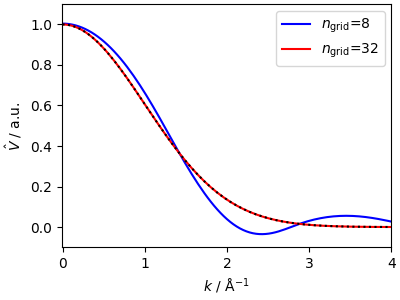
<matplotlib.legend.Legend object at 0x7f8edae1afd0>

An important consideration is that the splining of the k-space kernel requires a suitable grid. This is usually inferred from the real-space splining, but it is also possible to provided it as a further parameter to the constructor. If the analytical expression for \(\hat{V}(k)\) is known (and the spline is used for efficiency) one can also provide the values with the parameter yhat_grid

spline_kgrid = SplinePotential(
    r_grid=x_grid, y_grid=y_grid, k_grid=torch.linspace(0, 10, 32)
)
yhat_spline_kgrid = spline_kgrid.kernel_from_k_sq(k_test**2)

fig, ax = plt.subplots(1, 1, figsize=(4, 3), sharex=True, constrained_layout=True)

ax.plot(x_test, yhat_spline, "b-", label=r"automatic grid")
ax.plot(x_test, yhat_spline_kgrid, "b--", label=r"manual k-space grid")
ax.plot(k_test, yhat_test, "k:")
ax.set_xlabel(r"$k$ / Å$^{-1}$")
ax.set_ylabel(r"$\hat{V}$ / a.u.")
ax.set_xlim(-0.01, 4)
ax.set_ylim(-0.1, 1.1)
ax.legend()

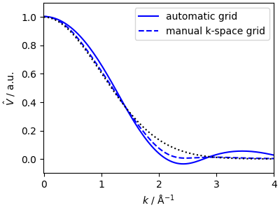
<matplotlib.legend.Legend object at 0x7f8edaec60d0>

Reciprocal grid and long-range potentials

torch-pme is all about long-range potentials, and the problem with them is that they converge to zero very slowly. In order to address this, SplinePotential implements a “reciprocal spline”, i.e. the splining grid provided in the definition of the potential is actually defined relative to \(1/r\), and “continued” to \(1/r\rightarrow 0\). We use a smeared-Coulomb potential to have a more interesting use case.

coulomb = CoulombPotential(smearing=1.0)
x_grid = torch.logspace(-2, 2, 100, device=device, dtype=dtype)
y_grid = coulomb.lr_from_dist(x_grid)

# create a spline potential
spline_direct = SplinePotential(r_grid=x_grid, y_grid=y_grid, reciprocal=False)
spline = SplinePotential(r_grid=x_grid, y_grid=y_grid, reciprocal=True)

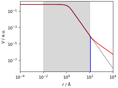
The “direct” spline fails miserably outside the fitting range, while the “reciprocal” spline extrapolates nicely.

t_grid = torch.logspace(-4, 4, 100)
z_coul = coulomb.lr_from_dist(t_grid)
z_direct = spline_direct.lr_from_dist(t_grid)
z_spline = spline.lr_from_dist(t_grid)

fig, ax = plt.subplots(
    1, 1, figsize=(4, 3), sharey=True, sharex=True, constrained_layout=True
)
ax.loglog(t_grid, z_direct, "b-", label="direct spline")
ax.loglog(t_grid, z_spline, "r-", label="reciprocal spline")
ax.loglog(t_grid, z_coul, "k:")
ax.set_xlabel(r"$r$ / Å")
ax.set_ylabel(r"$V$ / a.u.")
ax.axvspan(1e-2, 1e2, color="gray", alpha=0.3, label="fitted region")
ax.set_xlim(1e-4, 1e4)

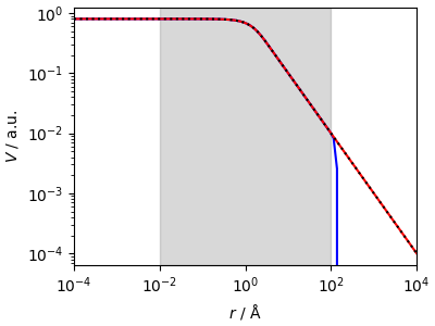
(0.0001, 10000.0)

This is good, but not magical, and if the tail behavior is not \(1/x\) the spline will only be able to approximate for a short segment (due to the continuity condition) but will eventually revert to an asymptotic \(1/r\) behavior. Still, this is much better than a direct spline.

y_grid_2 = y_grid**2
spline_2 = SplinePotential(r_grid=x_grid, y_grid=y_grid_2, reciprocal=True)
spline_2_direct = SplinePotential(r_grid=x_grid, y_grid=y_grid_2, reciprocal=False)
z_coul_2 = z_coul**2
z_spline_2 = spline_2.lr_from_dist(t_grid)
z_spline_2_direct = spline_2_direct.lr_from_dist(t_grid)

fig, ax = plt.subplots(
    1, 1, figsize=(4, 3), sharey=True, sharex=True, constrained_layout=True
)
ax.loglog(t_grid, z_spline_2_direct, "b-", label="direct spline")
ax.loglog(t_grid, z_spline_2, "r-", label="reciprocal spline")
ax.loglog(t_grid, z_coul_2, "k:")
ax.set_xlabel(r"$r$ / Å")
ax.set_ylabel(r"$V$ / a.u.")
ax.axvspan(1e-2, 1e2, color="gray", alpha=0.3, label="fitted region")
ax.set_xlim(1e-4, 1e4)

(0.0001, 10000.0)

Fourier-domain kernel

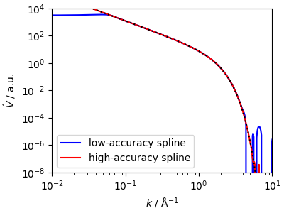
The calculation of a Fourier-domain kernel is a very delicate affair for a long-tail potential, which is apparent in the noisy behavior at high-\(k\), and the cutoff at the lowest point sampled at small wavevector. These numerical issues can be mitigated, but ultimately have low impact on the accuracy of models built on the splined potential.

Note that the initialization of the spline parameters and the calculation of the radial Fourier transform is run in double precision regardless of the type of the input grids. After initialization, further calculations are performed at the level corresponding to the grid precision.

spline = SplinePotential(r_grid=x_grid, y_grid=y_grid, reciprocal=True)

x_grid_hiq = torch.logspace(-4, 4, 1000, device=device, dtype=dtype)
y_grid_hiq = coulomb.lr_from_dist(x_grid_hiq)
spline_hiq = SplinePotential(r_grid=x_grid_hiq, y_grid=y_grid_hiq, reciprocal=True)

k_grid = torch.logspace(-4.1, 4, 1000)
krn_coul = coulomb.kernel_from_k_sq(k_grid**2)
krn_spline = spline.kernel_from_k_sq(k_grid**2)
krn_spline_hiq = spline_hiq.kernel_from_k_sq(k_grid**2)

fig, ax = plt.subplots(
    1, 1, figsize=(4, 3), sharey=True, sharex=True, constrained_layout=True
)


ax.loglog(k_grid, krn_spline, "b-", label="low-accuracy spline")
ax.loglog(k_grid, krn_spline_hiq, "r-", label="high-accuracy spline")
ax.loglog(k_grid, krn_coul, "k:")

ax.set_xlabel(r"$k$ / Å$^{-1}$")
ax.set_ylabel(r"$\hat{V}$ / a.u.")
ax.set_xlim(1e-2, 10)
ax.set_ylim(1e-8, 1e4)
ax.legend()

<matplotlib.legend.Legend object at 0x7f8eda973390>

Combining with Fourier filters and meshes

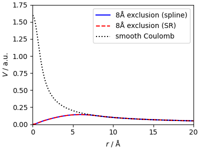
To see a potential application of this splining framework, consider the calculation of a “excusion-radius” Coulomb potential, i.e. a smooth Coulomb potential with the short-range region removed (so that) short-range structure does not contribute to the field around an atom.

Normally this is achieved through a short-range correction, that however can be cumbersome in some applications (e.g. if one wants to compute explicitly the potential on a grid).

smearing = 0.5
coulomb = CoulombPotential(smearing=smearing, exclusion_radius=None)
coulomb_exclude = CoulombPotential(smearing=smearing, exclusion_radius=8.0)

x_grid = torch.logspace(-3, 3, 1000)
y_grid = coulomb_exclude.lr_from_dist(x_grid) + coulomb_exclude.sr_from_dist(x_grid)

# create a spline potential for with the exclusion range built in
spline = SplinePotential(
    r_grid=x_grid, y_grid=y_grid, smearing=smearing, reciprocal=True, yhat_at_zero=0.0
)

The real-space part of the potential matches the reference and shows clearly how this eliminates the contribution from the atoms within a short-range cutoff. Here we use a very smooth cutoff, but one could as well use a much more aggressive cutoff function.

t_grid = torch.logspace(-3, 3, 1000)
y_bare = coulomb.lr_from_dist(t_grid)
y_exclude = coulomb_exclude.lr_from_dist(t_grid) + coulomb_exclude.sr_from_dist(t_grid)
y_spline = spline.lr_from_dist(t_grid)

fig, ax = plt.subplots(
    1, 1, figsize=(4, 3), sharey=True, sharex=True, constrained_layout=True
)
ax.plot(t_grid, y_spline, "b-", label="8Å exclusion (spline)")
ax.plot(t_grid, y_exclude, "r--", label="8Å exclusion (SR)")
ax.plot(t_grid, y_bare, "k:", label="smooth Coulomb")

ax.set_xlabel(r"$r$ / Å")
ax.set_ylabel(r"$V$ / a.u.")
ax.set_xlim(0, 20)
ax.set_ylim(0, 1.75)
ax.legend()

<matplotlib.legend.Legend object at 0x7f8eda85e850>

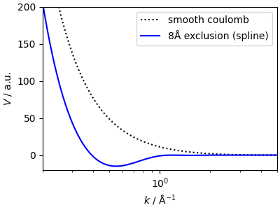
The k-space kernel has a non-trivial shape

k_grid = torch.logspace(-3, 3, 400)
krn_coul = coulomb.kernel_from_k_sq(k_grid**2)
krn_spline = spline.kernel_from_k_sq(k_grid**2)

fig, ax = plt.subplots(
    1, 1, figsize=(4, 3), sharey=True, sharex=True, constrained_layout=True
)
ax.semilogx(k_grid, krn_coul, "k:", label="smooth coulomb")
ax.semilogx(k_grid, krn_spline, "b-", label=r"8Å exclusion (spline)")
ax.set_xlabel(r"$k$ / Å$^{-1}$")
ax.set_ylabel(r"$V$ / a.u.")
ax.set_xlim(2e-1, 5)
ax.set_ylim(-20, 2e2)
ax.legend()

<matplotlib.legend.Legend object at 0x7f8eda8d4cd0>

Compute the real-space potential

Generate a trial structure – a distorted rocksalt structure with perturbed positions and charges

structure = ase.Atoms(
    positions=[
        [0, 0, 0],
        [3, 0, 0],
        [0, 3, 0],
        [3, 3, 0],
        [0, 0, 3],
        [3, 0, 3],
        [0, 3, 3],
        [3, 3, 3],
    ],
    cell=[6, 6, 6],
    symbols="NaClClNaClNaNaCl",
)
structure = structure.repeat([3, 3, 1])

displacement = torch.normal(mean=0.0, std=5e-1, size=(len(structure), 3), generator=rng)
structure.positions += displacement.numpy()

charges = torch.tensor(
    [[1.0], [-1.0], [-1.0], [1.0], [-1.0], [1.0], [1.0], [-1.0]] * 9,
    dtype=dtype,
    device=device,
).reshape(-1, 1)
charges += torch.normal(mean=0.0, std=2e-1, size=(len(charges), 1), generator=rng)
positions = torch.from_numpy(structure.positions).to(device=device, dtype=dtype)
cell = torch.from_numpy(structure.cell.array).to(device=device, dtype=dtype)

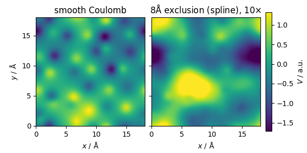
We use MeshInterpolator and KSpaceFilter to compute the potential on a grid. Note that the Coulomb potential includes only the k-space part, and therefore has no exclusion zone in reality.

ns = torchpme.lib.kvectors.get_ns_mesh(cell, smearing * 0.5)
mesh_interpolator = torchpme.lib.MeshInterpolator(
    cell=cell, ns_mesh=ns, interpolation_nodes=3, method="P3M"
)
kernel_exclusion = torchpme.lib.KSpaceFilter(
    cell=cell,
    ns_mesh=ns,
    kernel=coulomb_exclude,
    fft_norm="backward",
    ifft_norm="forward",
)

kernel_spline = torchpme.lib.KSpaceFilter(
    cell=cell,
    ns_mesh=ns,
    kernel=spline,
    fft_norm="backward",
    ifft_norm="forward",
)

mesh_interpolator.compute_weights(positions)
rho_mesh = mesh_interpolator.points_to_mesh(particle_weights=charges)
ivolume = torch.abs(cell.det()).pow(-1)

kernel_exclusion.update(cell, ns)
coulomb_mesh = kernel_exclusion.forward(rho_mesh) * ivolume

kernel_spline.update(cell, ns)
spline_mesh = kernel_spline.forward(rho_mesh) * ivolume

The potential computed using SplinePotential also takes into account the removal of the short-range part of the smooth Coulomb potential, and therefore describes only the slowly-varying part that is generated by the position and charge disorder.

fig, ax = plt.subplots(
    1, 2, figsize=(6, 3), sharey=True, sharex=True, constrained_layout=True
)
mesh_extent = [
    0,
    cell[0, 0],
    0,
    cell[1, 1],
]

z_plot = coulomb_mesh[0, :, :, 0].cpu().detach().numpy()
z_plot = np.vstack([z_plot, z_plot[0, :]])  # Add first row at the bottom
z_plot = np.hstack(
    [z_plot, z_plot[:, 0].reshape(-1, 1)]
)  # Add first column at the right

z_min, z_max = (z_plot.min(), z_plot.max())

cf_coulomb = ax[0].imshow(
    z_plot,
    extent=mesh_extent,
    vmin=z_min,
    vmax=z_max,
    origin="lower",
    interpolation="bilinear",
)

z_plot = spline_mesh[0, :, :, 0].cpu().detach().numpy()
z_plot = np.vstack([z_plot, z_plot[0, :]])  # Add first row at the bottom
z_plot = np.hstack(
    [z_plot, z_plot[:, 0].reshape(-1, 1)]
)  # Add first column at the right

cf_spline = ax[1].imshow(
    z_plot * 10,
    extent=mesh_extent,
    vmin=z_min,
    vmax=z_max,
    origin="lower",
    interpolation="bilinear",
)

ax[0].set_title("smooth Coulomb")
ax[1].set_title(r"8Å exclusion (spline), 10$\times$")
ax[0].set_xlabel(r"$x$ / Å")
ax[1].set_xlabel(r"$x$ / Å")
ax[0].set_ylabel(r"$y$ / Å")
fig.colorbar(cf_coulomb, ax=ax[1], label=r"$V$ / a.u.")
fig.show()