Optimizing a linear combination of potentials

Authors:

Egor Rumiantsev @E-Rum; Philip Loche @PicoCentauri

This is an example to demonstrate the usage of the CombinedPotential class to evaluate potentials that combine multiple pair potentials with optimizable weights.

We will optimize the weights to reporoduce the energy of a system that interacts solely via Coulomb interactions.

import ase.io
import chemiscope
import matplotlib.pyplot as plt
import torch
from vesin.torch import NeighborList

from torchpme import CombinedPotential, EwaldCalculator, InversePowerLawPotential
from torchpme.prefactors import eV_A

dtype = torch.float64

Combined potentials

We load the small dataset that contains eight randomly placed point charges in a cubic cell of different cell sizes. Each structure contains four positive and four negative charges that interact via a Coulomb potential.

frames = ase.io.read("coulomb_test_frames.xyz", ":")

chemiscope.show(
    frames=frames,
    mode="structure",
    settings=chemiscope.quick_settings(
        structure_settings={"unitCell": True, "bonds": False}
    ),
)

×

We choose half of the box length as the cutoff for the neighborlist and also deduce the other parameters from the first frame.

cutoff = frames[0].cell.array[0, 0] / 2 - 1e-6
smearing = cutoff / 6.0
lr_wavelength = 0.5 * smearing

We now construct the potential as sum of two InversePowerLawPotential using CombinedPotential. The presence of a numerical smearing value is used as an indication that the potential can compute the terms needed for range-separated evaluation, and so one has to set it also for the combined potential, even if it is not used explicitly in the evaluation of the combination.

pot_1 = InversePowerLawPotential(exponent=1, smearing=smearing)
pot_2 = InversePowerLawPotential(exponent=2, smearing=smearing)
pot_1 = pot_1.to(dtype=dtype)
pot_2 = pot_2.to(dtype=dtype)
potential = CombinedPotential(potentials=[pot_1, pot_2], smearing=smearing)
potential = potential.to(dtype=dtype)

# Note also that :class:`CombinedPotential` can be used with any combination of
# potentials, as long they are all either direct or range separated. For instance, one
# can combine a :class:`CoulombPotential` and a :class:`SplinePotential`.

Plotting terms in the potential

We now plot of the individual and combined potential functions together with an explicit sum of the two potentials.

dist = torch.logspace(-3, 2, 1000, dtype=dtype)

fig, ax = plt.subplots()

ax.plot(dist, pot_1.from_dist(dist), label="p=1")
ax.plot(dist, pot_2.from_dist(dist), label="p=2")

ax.plot(dist, potential.from_dist(dist).detach(), label="Combined potential", c="black")
ax.plot(
    dist,
    pot_1.from_dist(dist) + pot_2.from_dist(dist),
    label="Explict combination",
    ls=":",
)

ax.set(
    xlabel="Distance", ylabel="Potential", xscale="log", yscale="log", xlim=[1e-3, 1e2]
)

ax.legend()

plt.show()

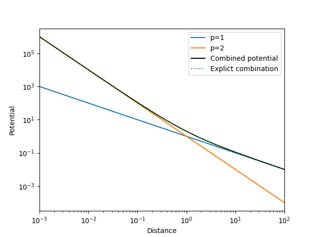
In the log-log plot we see that the \(p=2\) potential (orange) decays much faster compared to the \(p=1\) potential (blue). We also verify that the combined potential (black) is the sum of the two potentials that we explicitly calculated (dotted green line).

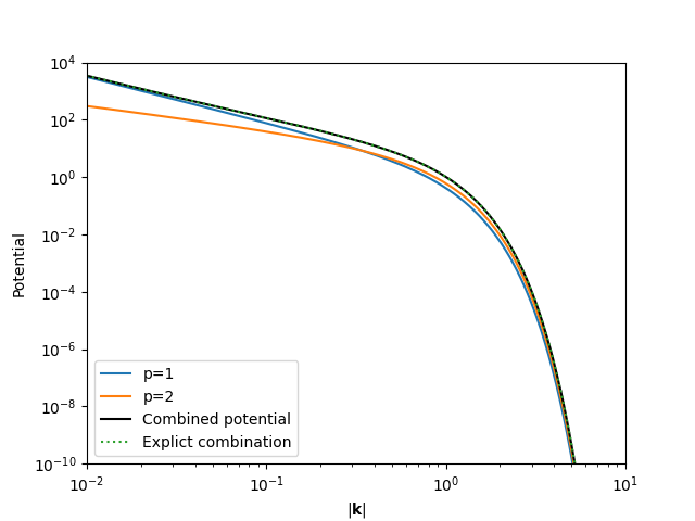
The CombinedPotential class combines all terms in a range-separated potential, including the k-space kernel.

k = torch.logspace(-2, 2, 1000, dtype=dtype)

fig, ax = plt.subplots()

ax.plot(dist, pot_1.lr_from_k_sq(k**2), label="p=1")
ax.plot(dist, pot_2.lr_from_k_sq(k**2), label="p=2")

ax.plot(
    dist, potential.lr_from_k_sq(k**2).detach(), label="Combined potential", c="black"
)
ax.plot(
    dist,
    pot_1.lr_from_k_sq(k**2) + pot_2.lr_from_k_sq(k**2),
    label="Explict combination",
    ls=":",
)

ax.set(
    xlabel=r"$|\mathbf{k}|$",
    ylabel="Potential",
    xscale="log",
    yscale="log",
    xlim=[1e-2, 1e1],
    ylim=[1e-10, 1e4],
)

ax.legend()

plt.show()

Optimizing the mixing weights

We next construct the calculator. Note that below we use the EwaldCalculator but one can of course also use the PMECalculator if one wants to optimize a much bigger system.

calculator = EwaldCalculator(
    potential=potential, lr_wavelength=lr_wavelength, prefactor=eV_A
)
calculator.to(dtype=dtype)

EwaldCalculator(
  (potential): CombinedPotential(
    (potentials): ModuleList(
      (0-1): 2 x InversePowerLawPotential()
    )
  )
)

To save some time during optimization we precompute the neighborlist and store all values in convient lists. We store the data in lists of torch tensors because in general the number of particles in each frame can be different.

nl = NeighborList(cutoff=cutoff, full_list=False)

l_positions = []
l_cell = []
l_charges = []
l_neighbor_indices = []
l_neighbor_distances = []
l_ref_energy = torch.zeros(len(frames))

for i_atoms, atoms in enumerate(frames):
    positions = torch.from_numpy(atoms.positions)
    cell = torch.from_numpy(atoms.cell.array)
    charges = torch.from_numpy(atoms.get_initial_charges()).reshape(-1, 1)

    p, d = nl.compute(points=positions, box=cell, periodic=True, quantities="Pd")

    l_positions.append(positions)
    l_cell.append(cell)
    l_charges.append(charges)

    l_neighbor_indices.append(p)
    l_neighbor_distances.append(d)

    l_ref_energy[i_atoms] = atoms.get_potential_energy()

Definition of loss and optimizer

For the optimization we define two functions that compute the energy of all structures and the mean squared error of the energy with respect to the reference values as loss.

def compute_energy() -> torch.Tensor:
    """Compute the energy of all structures using a globally defined `calculator`."""
    energy = torch.zeros(len(frames))
    for i_atoms in range(len(frames)):
        charges = l_charges[i_atoms]

        potential = calculator(
            charges=charges,
            cell=l_cell[i_atoms],
            positions=l_positions[i_atoms],
            neighbor_indices=l_neighbor_indices[i_atoms],
            neighbor_distances=l_neighbor_distances[i_atoms],
        )
        energy[i_atoms] = (charges * potential).sum()

    return energy


def loss() -> torch.Tensor:
    """Compute the mean squared error of the energy."""
    energy = compute_energy()
    mse = torch.sum((energy - l_ref_energy) ** 2)
    return mse.sum()


optimizer = torch.optim.Adam(calculator.parameters(), lr=0.1)

Running the optimization

We now optimize the weights of the potentials to minimize the mean squared error using the torch.optim.Adam optimizer and stop either after 1000 epochs or when the loss is smaller than \(10^{-2}\).

weights_timeseries = []
loss_timeseries = []

for _ in range(1000):
    optimizer.zero_grad()

    loss_value = loss()
    loss_value.backward()
    optimizer.step()

    loss_timeseries.append(float(loss_value.detach().cpu()))
    weights_timeseries.append(calculator.potential.weights.detach().cpu().tolist())

    if loss_value < 1e-4:
        break

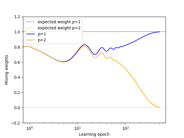
We can show the evolution of the weights during the optimization. The weights for the \(1/r\) and \(1/r^2\) potentials converge towards \(1\) and \(0\), respectively. This is the expected behavior, since the reference potential used to compute the energy of the structures includes only a Coulombic term.

fig, ax = plt.subplots()

ax.axhline(1, c="blue", ls="dotted", label="expected weight p=1")
ax.axhline(0, c="orange", ls="dotted", label="expected weight p=2")

weights_timeseries_array = torch.tensor(weights_timeseries)

ax.plot(weights_timeseries_array[:, 0], label="p=1", c="blue")
ax.plot(weights_timeseries_array[:, 1], label="p=2", c="orange")

ax.set(
    ylim=(-0.2, 1.2),
    xlabel="Learning epoch",
    ylabel="Mixing weights",
    xscale="log",
)

ax.legend()
plt.show()